In spring and fall 2005, cross- and along-shelf transects were sampled to evaluate the influence of physical forcing, including sea ice, tides, and winds, on the lower trophic levels of the Bering Sea ecosystem. The hydrography, nutrients, chlorophyll, and zooplankton abundance and species composition were all affected by the presence or absence of sea ice on a north–south transect along the 70-m isobath. In May, shelf waters between ~59°N and 62°N were cold and relatively fresh, and benthic invertebrate larvae and chaetognaths were a significant fraction of the zooplankton community, while to the south the water was warmer, saltier, and the zooplankton community was dominated by copepods. The position of the transition between ice-affected and ice-free portions of the shelf was consistent among temperature, salinity, nutrients, and oxygen. This transition in the hydrographic variables persisted through the summer, but it shifted ~150 km northward as the season progressed. While a transition also occurred in zooplankton species composition, it was farther north than the physical/chemical transition and did not persist through the summer. Mooring data demonstrated that the change in the position of the transition in physical and chemical properties was due to northward or eastward advection of water onto and across the shelf. From south to north along the 70-m isobath, tidal energy decreased, resulting in a less sharply stratified water column on the northern portion of the middle shelf, as opposed to a well-defined, two-layered system in the southern portion. This more gradual stratification in the north permitted a greater response to mixing from winds, which were homogeneous from north to south. Thus the physical and biological structure at any one location over the middle shelf is dynamic over the course of a year, and results from a combination of in situ processes and climate-mediated regional forcing which is dominated in most years by sea ice.
The high subarctic seas (Norwegian/Barents Sea, Labrador Sea, and Bering Sea) are characterized by high biological productivity and the seasonal presence of sea ice (Hunt and Drinkwater, 2005). Differences in physiography and orientation or exposure to the dominant forcing mechanisms help to determine the landscape ecology of these areas (Bailey et al., 2003; Ciannelli and Bailey, 2005; Stabeno et al., 2006). In the last decade, global temperatures have reached some of the highest levels ever recorded and projections of future (after 2030) temperature suggest that the greatest rates of change will be at high latitudes (IPCC, 2007). Increases in global temperatures have begun to affect the areal extent, concentration, and thickness of ice in both the polar regions and in the subarctic seas (IPCC, 2007). It is imperative that we understand the role played by physical mechanisms in arctic ecosystems, including how sea ice impacts the structure, function, and productivity of these ecosystems. The focus of this article is an examination of the physics, chemistry, chlorophyll, and zooplankton over the eastern Bering Sea shelf from spring through summer 2005. Since 2005 was a particularly warm year in the Bering Sea, it may provide insight into the future of the Bering Sea ecosystem.
Sea ice is a critical component of the oceanography of the Bering Sea shelf. During winter, frigid winds blow southward over the eastern Bering Sea, forming ice in the lee of headlands and islands. In these ice-free areas or polynyas, brine rejection results from ice formation and dense, saline water sinks to the bottom of the shallow shelf. The sea ice formed in the polynyas is transported southward by the wind. The leading edge melts as it encounters warmer (>0°C) water, thereby cooling and freshening the water column. The thickness, areal coverage, and southernmost extent of sea ice vary on multiple timescales: year-to-year, quasi-decadal, and long-term trends (Niebauer et al., 1999; Wyllie-Echeverria and Ohtani, 1999; Stabeno et al., 2007). In recent decades, the southernmost extent of sea ice was a maximum in the early- to mid-1970s, and a minimum in the early 2000s (Stabeno et al., 2007). In a heavy ice year (e.g., 1975/1976), ice can be advected southward almost to Unimak Pass (54.5°N; Fig. 1) and be present in the north from mid-November until late June. In light ice years (e.g., 2005), the maximum southern extent remains north of the Pribilof Islands (57°N), but can still persist over the northern shelf (north of at 62°N) into June. Recent minima in ice extent are thought to be a response to global climate change and decadal variability (Overland and Stabeno, 2004). The years 2000–2005 were among the warmest on record in the area; winter ocean temperatures stayed above 0°C over the southern shelf (south of 58°N), and in 2005 the depth-averaged water temperature during summer approached 8°C on the southeastern middle shelf. During 2000–2005, shelf temperatures were 2–3°C warmer than those observed in the 1990s and these relatively warm temperatures were a direct response to the atmospheric circulation patterns and reduction in ice cover (Stabeno et al., 2007).
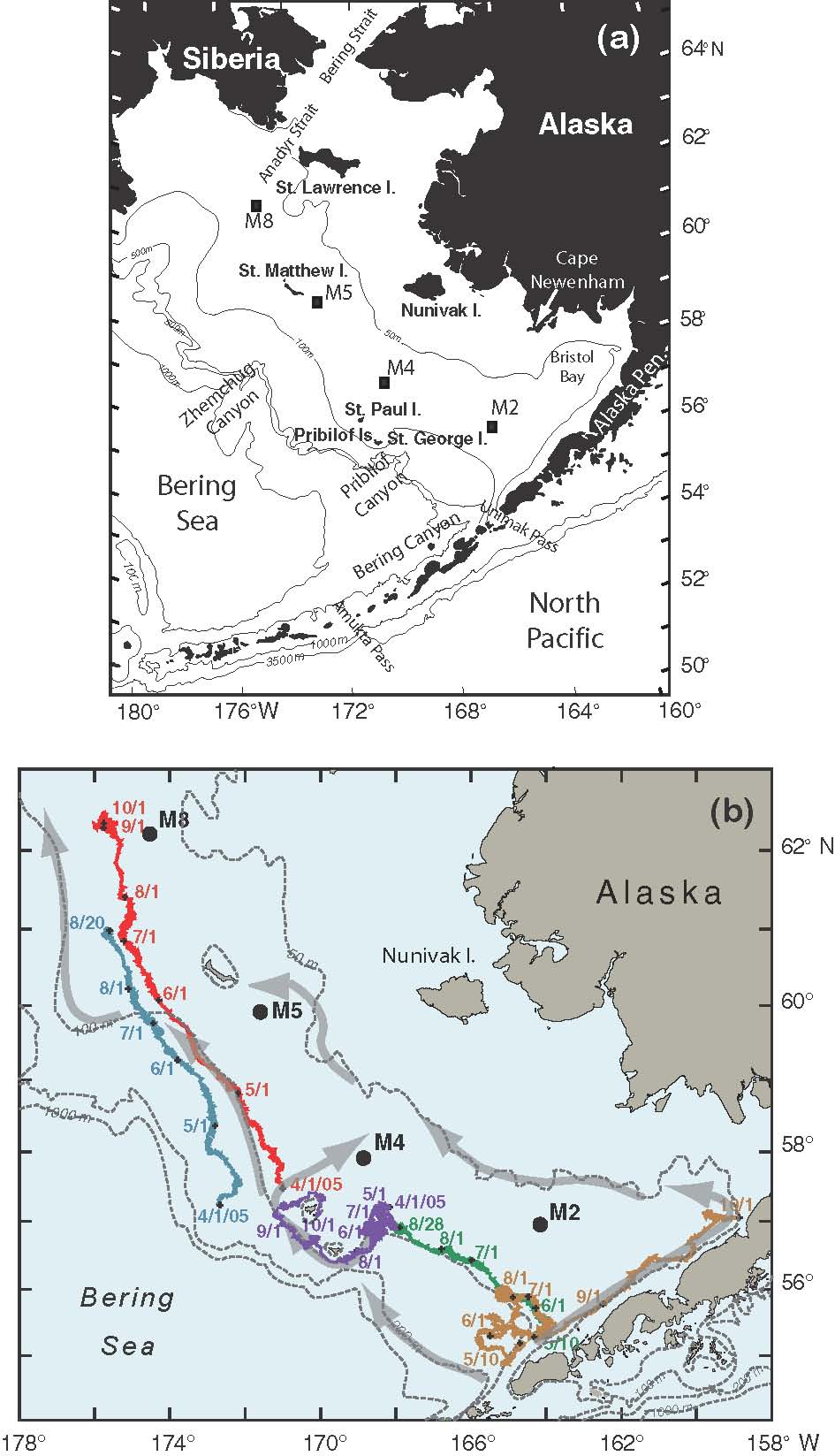
Fig. 1. (a) A map of the study region with bathymetric and geographic labels. (b) The locations of the four primary moorings (M2, M4, M5, and M8) are indicated. The arrows represent the mean flow over the shelf. Also shown are the trajectories from a series of drifters that were deployed in the region. The date of deployment for each drifter is given at the beginning of each trajectory and the position at the beginning of each month is indicated by month/day.
The geographic focus of this paper is the broad eastern shelf. The shelf is ∼500 km wide and slopes gently from the coast westward to the shelf break at ∼180 m. The breadth and flatness of this shelf permits the formation of well-defined, cross-shelf domains. During summer, the eastern shelf south of 62°N is divided into three cross-shelf hydrographic and biological regions: the coastal domain (< 50 m water depth), which is vertically well-mixed by tidal and wind mixing; the middle shelf domain (∼50–100 m), which is sharply stratified into an upper mixed layer (winds) and a lower mixed layer (tides); and the outer shelf domain (∼100–180 m), where the surface wind-mixed layer and the bottom tidally mixed layer are separated by a transitional layer (Coachman, 1986; Kachel et al., 2002). Each of the regions has its own chemical signature (Whitledge et al., 1986; Sullivan et al., 2008), biological communities, and levels of lower trophic-level production (Cooney and Coyle, 1982; Sambrotto et al., 1986; Schneider et al., 1986; Smith and Vidal, 1986; Coyle et al., 1996; Springer et al., 1996).
The eastern Bering Sea shelf also has considerable along-shelf variability, and changes in climate will likely impact the hydrographic and biological differences between the southern and northern regions. For instance, at present, primary production supports a predominantly pelagic food web in the southern portion of the shelf, and a predominantly benthic food web in the northern portion of the shelf (Walsh and McRoy, 1986; Hunt et al., 2002; Grebmeier et al., 2006; Grebmeier and Barry, 2007). Therefore, climate-induced changes in the physical forcing of primary production could have varying effects on these different communities and portions of the shelf depending on the underlying food webs. There are already indications of changes in the northern portion of the shelf south of St. Lawrence Island, and in the Chirikov Basin between St. Lawrence Island and Bering Strait (Grebmeier et al., 2006). Studies begun in the mid-1980s have shown declines in the biomass (Sirenko and Koltun, 1992; Grebmeier, 1993; Grebmeier and Dunton, 2000; Grebmeier et al., 2006) and mean sizes of the dominant bivalves in the area (Lovvorn et al., 2003). The flux of carbon to the benthos in this region is related to a number of factors, including the timing of the ice-edge spring phytoplankton bloom and the seasonal transport of nutrients into the region by the Anadyr Current (Grebmeier et al., 2006).
Our objective for this paper is to describe and compare the underlying mechanisms and processes that distinguish the physics, chemistry, and biology of the northern and southern portions of the eastern middle shelf and the transitional area that lies between them. We consider only that part of the shelf south of ∼62.5°N and exclude the region around and north of St. Lawrence Island which is dominated by the flow through Bering Strait. A latitude of ∼63°N is the northern extent of the middle shelf domain. The area north of that latitude is predominantly shallower than 50 m and the physical and biological processes there may be more similar to the waters in the Chukchi Sea (north of Bering Strait) than they are to processes occurring in the Bering Sea to the south. The ultimate goal is to begin to understand the forces structuring the benthic-dominated northern shelf and the more pelagic-dominated southern shelf so that we can begin to predict how climate change and climate variability will impact the living marine resources of the eastern Bering Sea. Primarily, we use data from two cruises in 2005 (one in the early to mid-spring and the other in late summer/early fall), and data from a series of four moorings on the middle shelf. We begin with an examination of the ice cover and retreat during 2005. Next we compare the spatial patterns in hydrography, chemistry, and biology along the 70-m isobath and how they differed in the spring and late summer. We explore cross-shelf differences using an east–west transect just south of St. Matthew Island. The data from four biophysical moorings provide information on temporal variability of properties between the two cruises. Data from the moorings also reveal the role of currents, especially tidal mixing, on the structure and processes that occur over the shelf.
This study uses hydrographic data collected during two cruises in 2005—one on the R/V Thomas G. Thompson (cruise TN179 leg 3: 10 May–25 May) and the second on the NOAA ship Miller Freeman (MF05-13: 21 September–4 October). Conductivity-temperature-depth (CTD) measurements were collected with a Seabird SBE911 plus system (reference to trade names does not imply endorsement by NOAA) with dual temperature and salinity, oxygen (one SeaBird SBE 43 on TN179 and two on MF05-13), solar radiation (Biospherical PAR QSP-200L, 400–700 nm), and chlorophyll fluorescence sensors (WETStar WS3S). Fluorescence from both the moored fluorometers and the fluorometer on the CTD was converted to chlorophyll concentration (μg 1−1) using the relationships provided by the manufacturer for each instrument during annual service and calibration. Data were recorded during the downcast, with a descent rate of 15 m min−1 to a depth of 35 m, and 30 m min−1 below that. Salinity calibration samples were collected on most casts and analyzed on a calibrated laboratory salinometer. The distance between stations along the 70-m isobath and on the cross-shelf transects was ~20 km. Each cruise occupied the same CTD stations along the 70-m isobath.
During both cruises, water samples for dissolved inorganic nutrients were collected at each station using Niskin bottles. Nutrient samples were analyzed onboard for dissolved phosphate, silicic acid, nitrate, nitrite, and ammonia (only during TN179) using protocols of Gordon et al. (1993) and the ammonia protocol available at http://chemoc.coas.oregonstate.edu/~lgordon/cfamanual/whpmanual.pdf.
In situ oxygen sensors were calibrated by the manufacturer prior to each cruise, but a titrator was not available for ground truth measurements during the cruises. On TN179 there was one sensor, while on MF05–13 there were two sensors. The mean difference between the two sensors on each cast ranged from 3.9 to 6.7, with a mean of 5.6, and for each cast the correlation between the two sensors was greater than 0.99. We recognize the problem of not having titrated water samples for in situ calibration, but feel that the oxygen values provide patterns of variability that are informative and important in our descriptions of conditions on the shelf.
The modeled winds were estimated using daily data from the National Centers for Environmental Prediction (NCEP)/National Center for Atmospheric Research (NCAR) Reanalysis (Kalnay et al., 1996). We follow the procedure used in Bond and Adams (2002) to specify particular elements of the atmospheric forcing on a daily basis for selected periods and interpolated wind velocity to the locations of two moorings, M2 and M8 (Fig. 1). The daily winds from the reanalysis are reliable in this region (Ladd and Bond, 2002). Meteorological variables, including wind velocity, were also measured on the surface mooring at M2 as described below.
Four biophysical mooring sites (M2, M4, M5, and M8) are the cardinal locations of our observing network (Fig. 1). The moorings are recovered and redeployed twice a year, once in the spring (April/May) and again in the late summer or early fall (September/ October). Moorings at M2 have been maintained almost continuously since 1995. In addition, a series of moorings have been deployed at M4 since 1996 (continuous since 2000). M5 and M8 have been maintained since 2005 (current measurements since 2004) and 2004, respectively.
The main mooring at each site is constructed of heavy chain to protect it from loss due to sea ice and the heavy fishing pressure in the region. In 2005, data collected by instruments on the moorings included temperature (miniature temperature recorders, SBE-37 and SBE-39), salinity (SBE-37), nitrate (In Situ Ultraviolet Spectraphoto-meter, discussed below), and chlorophyll fluorescence (WET Labs DLSB ECO Fluorometer). Currents were measured using an upward-looking, bottom-mounted, 300 kHz Teledyne RD Instruments acoustic Doppler current profiler (ADCP) deployed next to the main mooring. All instruments were prepared, calibrated prior to deployment, and the data were processed according to manufacturer's specifications.
In 2005, we used an In Situ Ultraviolet Spectrophoto-meter (ISUS; Satlantic, Inc.) to estimate dissolved inorganic nitrate at M2. This instrument can sample hourly for as long as 12 months. ISUS uses optical technology (UV spectra) to provide chemical-free measurements of in situ nitrate and has been field tested on drifting buoys, towed vehicles, moorings, and CTD profilers. The instrument is solid state with no moving parts and has a sensitivity of 0.25 lM and 1% accuracy with post-processed CTD corrections. A discrete sample collected at the mooring site in May agreed to within 0.4 lM of the ISUS measurement. Data were collected hourly.
The depths of the shallowest instruments on the main moorings vary from 1 to 20 m dependent upon the mooring location and the time of year (http://www.pmel.noaa.gov/foci/foci_moorings/mooring_info/mooring_location_info.html). When the mixed layer shoals above 11 m, the upper mixed layer measurements in the summer are sometimes under-represented in our data set (Stabeno et al., 2007). Sampling intervals varied for the different instruments and range from every 10 min to once an hour. During late spring and summer (the ice-free period), the mooring at M2 included a surface toroid buoy with an aluminum tower where a full suite of meteorological variables was collected (Gil WindSonic for winds, Vaisal HMP-50 for air temperature and humidity, Setra 270 for atmospheric pressure and Eppley BSP for PAR). Winds were measured at a height of ~3 m. This surface mooring also permitted measurement of ocean temperature and salinity at ~1 m.
Samples for mesozooplankton were collected using double-oblique tows of paired bongo frames (60-cm frame with 0.333 mm mesh and 20-cm frame with 0.150 mm mesh). Tows extended from the surface to within 5 m of the bottom. A SeaBird SeaCat SBE19-plus was attached above the top bongo frame and telemetered net depth in real time to the operator. Each net mouth contained a calibrated General Oceanics mechanical flow meter. The samples were preserved in a sodium borate buffered 5% formalin: seawater solution and then sent to the Polish Plankton Sorting and Identification Center (Szczecin, Poland) for processing. Organisms were identified to the lowest possible taxonomic level and then enumerated. All enumerated organisms were returned to AFSC in Seattle, Washington, for quality control.
We used weekly data on ice extent and concentration from the National Ice Center (NIC). The NIC published a CD of ice extent and concentration from 1972 to 1994. The CD specifies ice concentration and extent in 0.25° latitude and longitude bins. After a break of several years, the NIC resumed posting ice concentration information in GIS format on their websites (http://www.natice.noaa.gov/pub/Archive/arctic/ and http://www.natice.noaa.gov/products/archi/index.htm). Data from 1995 to 2006 were converted to 0.25° bins to make them comparable to the earlier (1972–1994) data. The NIC assimilates data from satellites (Radarsat, Defense Meteorological Satellite Program, and Envisat) as well as aerial reconnaissance, local information, climatology, meteorological information, and models to produce their estimates of sea-ice extent and concentration.
In the southeastern Bering Sea, 2005 was a period of belowaverage seasonal sea-ice coverage and above-average air and water temperatures (Stabeno et al., 2007). In the last 36 years, the mid-1970s had the greatest ice cover in the southeastern Bering Sea (Fig. 2), while the seasonal sea-ice cover in the early 2000s was well below the 36-year mean. The average ice extent over the northern shelf, however, was not markedly different from the earlier "cold" period. This is not to say that there were not differences in ice thickness or spatial patterns of advance and/or retreat (e.g., Grebmeier et al., 2006), but rather in the broadest sense, the areal coverage of sea ice over the northern shelf has not varied on decadal scales. While some of the maxima and minima in the two series are coincident, the overall correlation of areal ice extent between the two areas was not statistically significant (99% significance).

Fig. 2. Average percent ice cover in two bands of latitude, 62–63°N and 57–58°N, that stretch from the coast to the International Date Line and the shelf break, respectively. Averages were calculated from US National Ice Center data for each winter–spring (December, January–May), 1972 through 2005.
During 2005, the maximum southern ice extent reached ~57°N on 11 April (almost a month prior to the spring cruise) with the edge stretching from Cape Newenham across the International Date Line to the Russian Federation (Fig. 3). By the beginning of the cruise (9 May) there had been significant melting of sea ice in Bristol Bay and the southern half of the 70-m isobath transect (Stations 88–118) and the southernmost cross-shelf transect were ice-free. Stations 60–68 in the lee of St. Lawrence Island were also ice-free. As the cruise progressed, the ice-free region to the west of St. Lawrence Island expanded to the southwest. Toward the end of the cruise, the ice barely reached the 70-m isobath stations (Fig. 3c). The eastern portion of the east-west transect located south of St. Matthew Island bordered the ice, but the western portion had been ice-free for several weeks (Fig. 3)
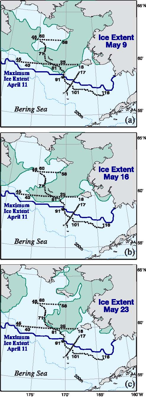
Fig. 3. Spring sea-ice extent during a three-week period in 2005. (a) Ice extent at the start of the cruise, (b) midway and (c) near the end of the cruise. The maximum ice extent was on April 11 and is shown as a thick black. The hydrographic stations for the spring cruise are indicated. The fall cruise occupied the same stations along the 70-m isobath. Moorings M4, M5, and M8 are at the intersection of the crossshelf lines and the 70-m isobath. M2 is at the southern terminus of the 70-m isobath.
The 70-m isobath is at the center of the middle shelf domain, and as such it is characterized by a two-layer structure during the late spring and summer, with ice playing an important role in determining its temperature and salinity. Our horizontal resolution of small features was limited by ~20 km station separation. The southern part of the 70-m transect was ice free the entire winter and spring of 2005, while over the northern portion the ice had retreated just the week prior to sampling. Maximum ice extent was near Station 91 (Fig. 3). As a result the water was warmer south of Station 91 than north of it (Fig. 4). There was a front (a change of ~2°C and 0.4 psu over a distance of ~40 km) between the fresher, colder northern waters and the more saline, warmer southern shelf waters. While the front persisted into September, its location migrated northward ~150 km, as did southern boundary of the cold pool (bottom water <2°C; Fig. 5). In September, the northern and southern regions of the middle shelf were distinguished by surface salinity, not surface temperature, and by bottom temperatures (Figs. 4 and 5).
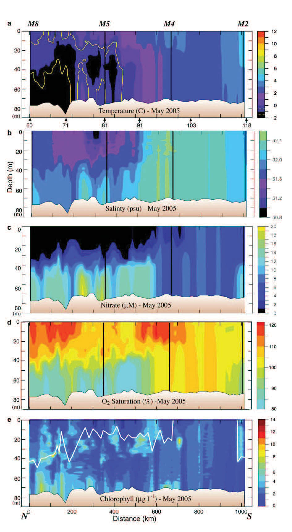
Fig. 4. Data collected along the 70-m isobath during the May 2005 cruise. The y-axes are depth. (a) Temperature, (b) salinity, (c) nitrate, (d) percent oxygen saturation and (e) chlorophyll. The vertical black lines indicate the position of the moorings. The distance between stations was ~20 km. The locations of specific stations are indicated at the bottom of the top panel. Nitrate was measured every ~10 m and at the bottom of each hydrographic cast. Since the stratification in the top panel was relatively weak, the 1°C isotherm is shown in yellow, and the −1°C isotherm is shown in white. The white line in the bottom panel is the mixed-layer depth (defined as the depth at which the temperature had decreased by 0.2°C).
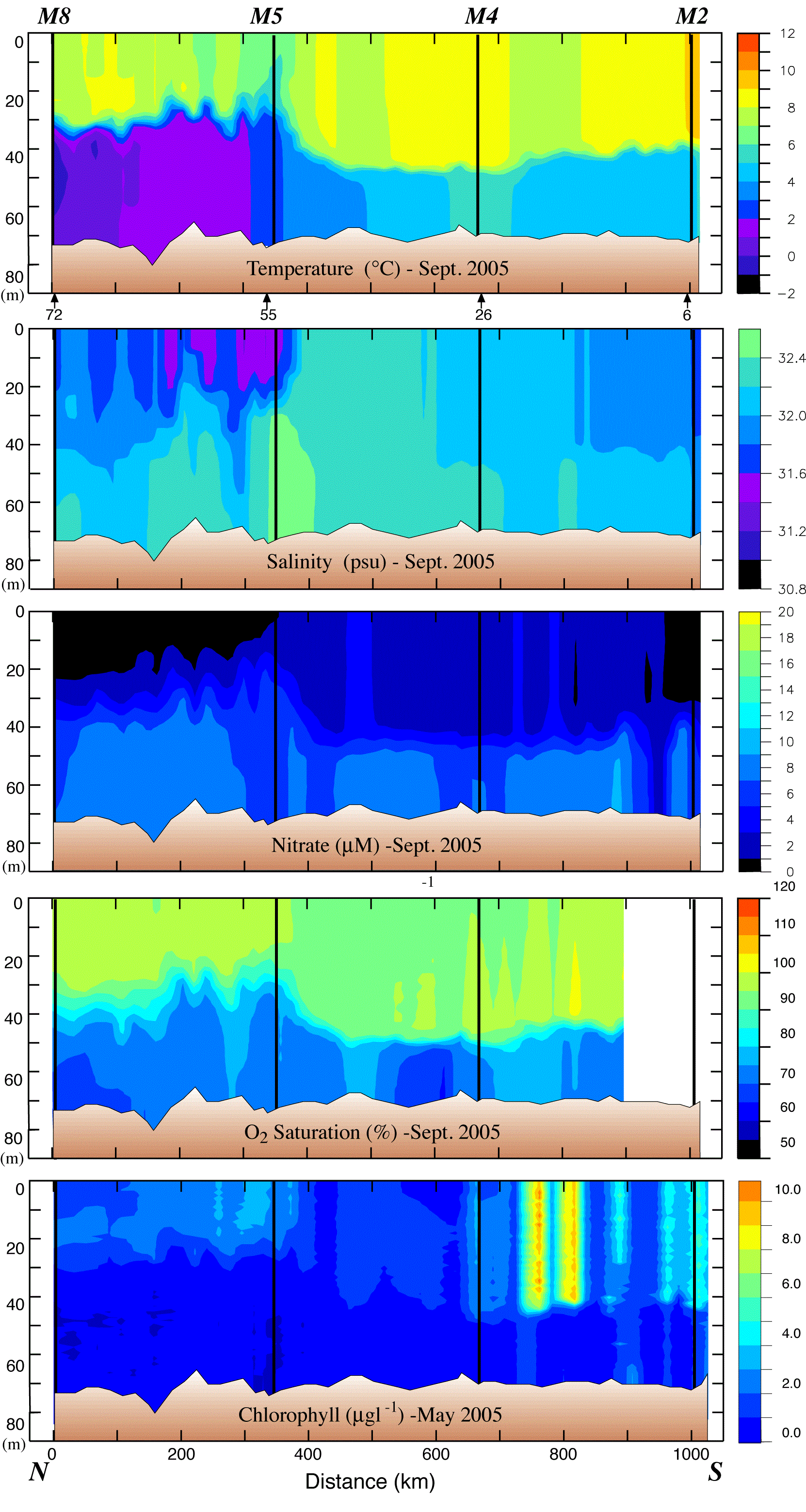
Fig. 5. Data collected along the 70-m isobath during the September 2005 cruise. The y-axes are depth. (a) Temperature, (b) salinity, (c) nitrate, (d) percent oxygen saturation and (e) chlorophyll. The black lines indicate the position of the moorings. The distance between stations was ~20 km. The locations of specific stations are indicated at the bottom of the top panel. Nitrate was measured every ~10 m and at the bottom of each cast.
During May, the vertical stratification south of the maximum ice extent was very weak, while north of maximum ice extent, stratification was stronger and almost totally a result of salinity (Fig. 6a). The greatest density difference between near-surface waters (5 m) and near-bottom waters (65 m) was found at x = ~300 km, where the ship sampled along the ice edge. While the density difference between 5 and 65 m was largest along the ice edge, the gradient was significant throughout the water column (Fig. 6b). By September, this pattern had changed markedly; the density difference between the top and the bottom of the water column was greatest over the northern shelf, where temperature and salinity contributed almost equally to the vertical density difference (Fig. 6c). The difference between the near-surface and near-bottom density over the southern shelf was mostly due to temperature. Along the portion of the 70-m isobath south of St. Matthew Island (~400 km in Fig. 6c) the stratification was limited to an extremely sharp interface at a depth of 40–50 m evident in the Brunt–Väisälä frequency (Fig. 6d), while the portion north of the island, the interface was more diffuse, with greatest gradient in density occurring at ~30 m (Figs. 5 and 6). The horizontal change in the intensity of the Brunt–Väisälä frequency (Fig. 6b and d) coincides with the front between northern and southern parts of the shelf.
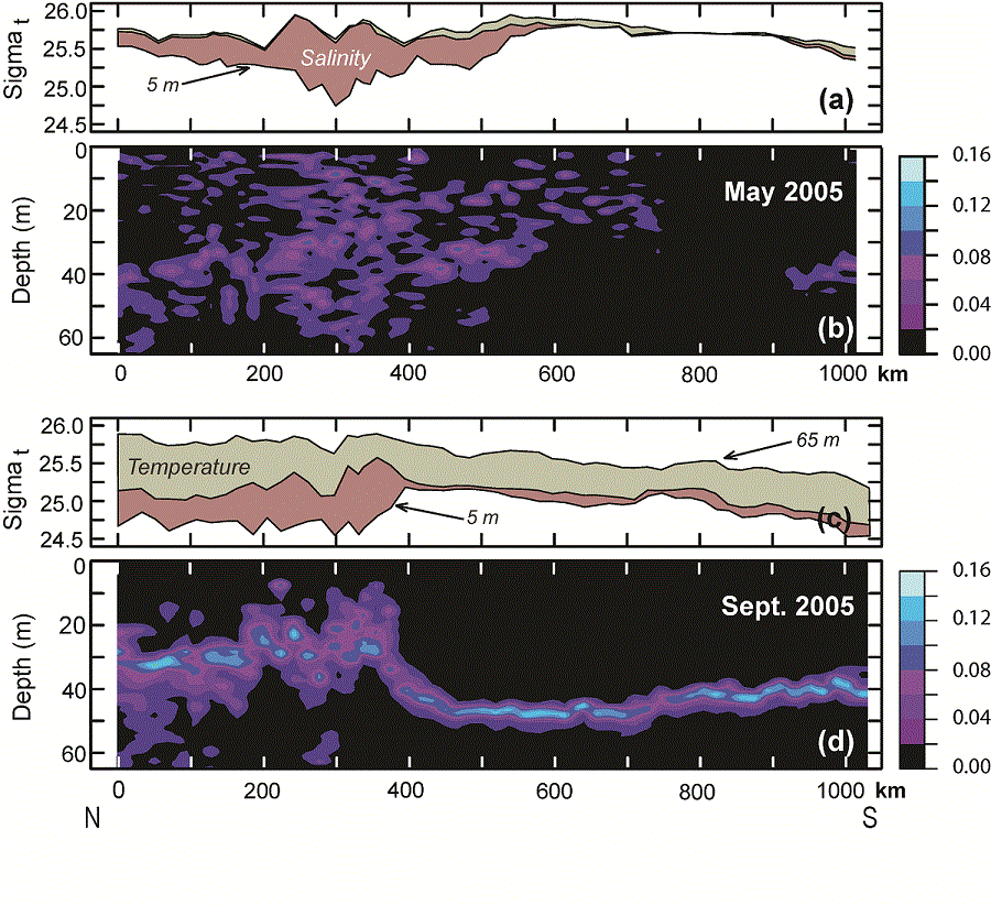
Fig. 6. Panels a and c: Sigma-t along the 70-m isobath at 5 m and at 65 m. The rose shaded area indicates the portion of difference between the near-surface and near-bottom densities that resulted from just salinity and the gray-green shade indicates the portion that resulted from temperature. Panels b and d: Contours of the Brunt–Väisälä frequency along the 70-m isobath in May and in September.
The maximum extent of ice in spring sets up chemical and biological fronts as well as physical fronts. The timing of the spring phytoplankton bloom is dependent upon the flux of solar energy, the presence/absence of ice, and the onset of water-column stratification. Along the northern portion of the 70-m isobath transect, a bloom had already occurred before the May cruise, with the highest spring chlorophyll found below the mixed layer and/or near the bottom (Fig. 4). The surface layer was depleted of nitrate and supersaturated with oxygen. The bottom layer was replete with nitrate, and had some of the highest concentrations of chlorophyll observed on the transect, while dissolved oxygen was under-saturated. This suggests that a significant fraction of the spring new production had sunk to the bottom, avoiding immediate consumption by micro- and mesozooplankton in the upper water column. The association of this bloom with ice will be discussed later using data from the moorings.
Historically, nitrate concentrations over the southern portion of the middle shelf prior to the spring bloom are 15–20 μM (Stabeno et al., 2002). The nitrate concentration in spring 2005 was approximately half that (the other macro-nutrients were similarly reduced), indicating that new production had already begun drawing down the nutrients even though the water column did not exhibit physical stratification. At the southernmost extent of the transect the water column was beginning to stratify and new production was occurring, as evidenced by declining nitrate concentrations and increased chlorophyll (Figs. 4 and 5). The timing of the blooms is discussed in more detail in the section on time series.
During late September, nitrate depletion was observed in the surface mixed layer at the northern end of the transect, but the region of depletion was smaller than observed in the spring. Because chlorophyll was low and oxygen was under-saturated, nitrate depletion in the north was most likely a remnant of spring and summer production. To the south of M5, nitrate concentrations were slightly higher (>1 μM), but chlorophyll and oxygen saturation remained low, suggesting low levels of new production. One exception was a region between M4 and M2 where temperatures were slightly cooler and chlorophyll concentrations were the highest observed in September. This would be consistent with a recent mixing event that introduced colder, nutrient-rich bottom water into the euphotic zone, promoting new production (Sambrotto et al., 1986). Historically, this portion of the 70-m isobath has shown considerable small-scale (~20 km) spatial variability (Stabeno et al., 2002). In addition, oxygen was not supersaturated (except at one station), suggesting that the rates of exchange with the atmosphere were high and/or primary production had recently increased, perhaps representing the early stages of the fall bloom at this locale (the fall bloom at M2 began in August, discussed below).
In September 2005, while ammonium concentrations in the upper water column of the 70-m isobath transect were low, concentrations in the bottom layer often exceeded 8 μM (Fig. 7). It has been previously observed that ammonium concentrations over the middle shelf have strong seasonal dependence and can be extremely high during the summer (Whitledge et al., 1986; Mordy et al., 2008; Rho et al., 2005). The high nitrite concentrations (often >1 μM) that we observed, however, have not been previously reported. The high nitrite concentrations observed in a few stations south of M5 were coincident with a comparable decrease in ammonium of ~2 μM. Nitrite concentrations in the world's oceans are almost always <1 μM and those observed in 2005 in the Bering Sea are comparable to concentrations observed in oxyclines of the equatorial Pacific Ocean. Nitrite is an intermediate formed during nitrification (the oxidation of ammonium to nitrate). High nitrite coincident with decreasing ammonium in well-oxygenated water suggests a decoupling of the oxidation steps associated with nitrification. While there are not enough data to develop a robust hypothesis on why such high concentrations of nitrite occurred in 2005, these unusual concentrations are an indication that the microbial ecosystems were perturbed in late summer 2005.
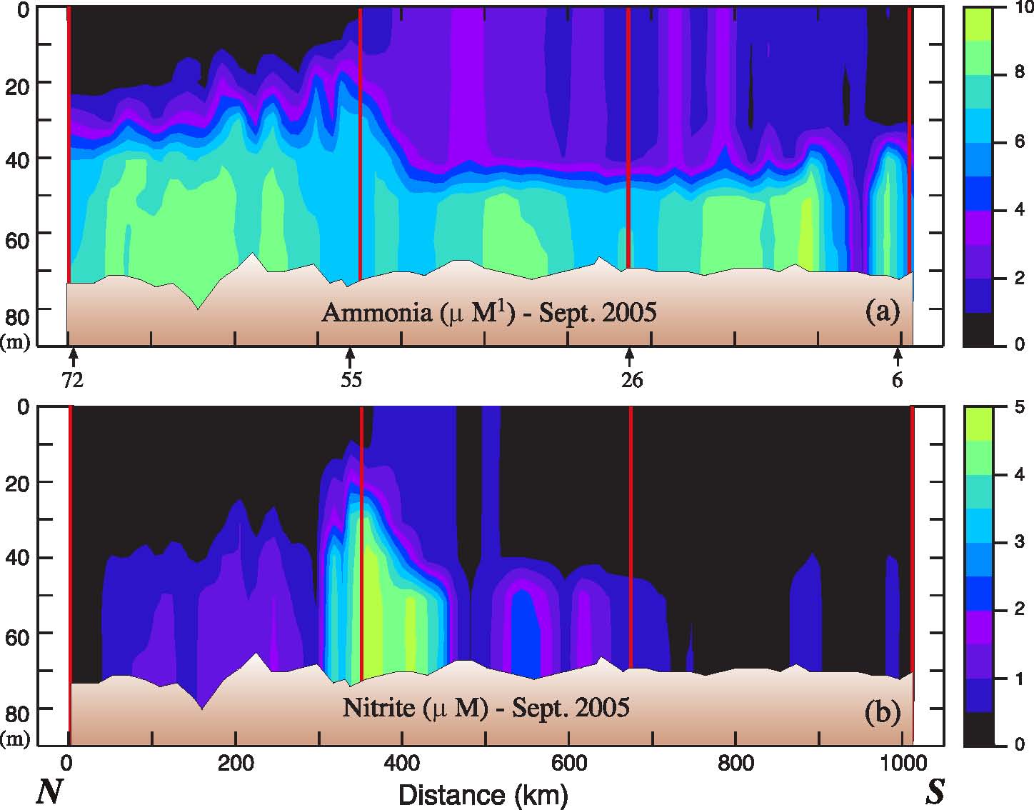
Fig. 7. (a) Ammonium and (b) nitrite in September 2005 along the 70-m isobath. The y-axes are depth. The vertical red lines indicate the position of the moorings.
In the spring and late summer, there were also differences in the community composition of zooplankton between the two regions as sampled by both the fine and coarse mesh nets (Fig. 8). In the spring, the contribution of Acartia spp. to total abundance was higher at the northernmost stations than at the southern stations. The five northern stations were also notable for the percent of total abundance contributed by chaetognaths (two stations) and barnacle nauplii (Cirripedia, two stations). These first five stations coincided with the area of very cold ocean temperatures ( 1°C, Fig. 4). Between 200 and 600 km, the community was dominated by Pseudocalanus spp. copepodites (
 70% total). At the last two stations along the transect, the percent of total abundance contributed by larvacea increased and Pseudocalanus spp. decreased. Throughout the transect, the relative contribution of copepodites of Calanus marshallae was small, with the highest concentrations of this important species found at the southern edge of the very cold region (not shown). Of the organisms enumerated from coarser mesh nets (333 μm), chaetognaths were relatively more important in the north than the south and Anomura (crab larvae), Neocalanus spp. and fish larvae contributed more to the total abundance in the south than the north (not shown).
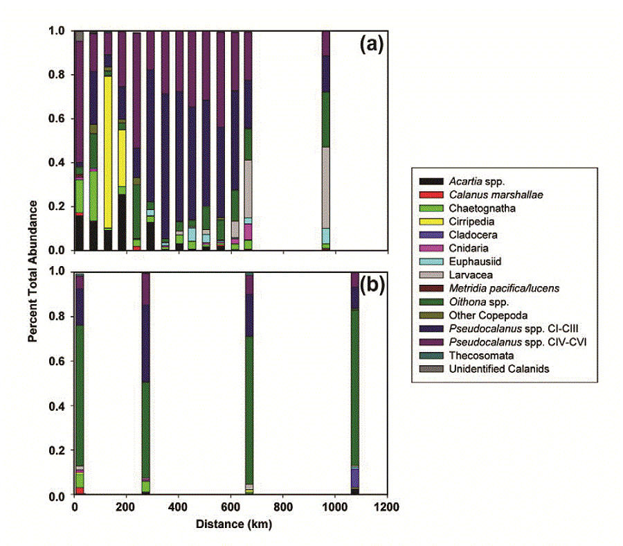
Fig. 8. Percent total abundance of common zooplankton along the 70-m isobath. (a) spring, (b) late summer. A single sample was obtained at every other station along the isobath during spring, but in the late summer, replicate samples were obtained at the mooring site and at four stations forming a square around the mooring site (total of five stations). The exception is at M8 where a storm forced us to end operations early. A single sample was collected at that mooring site.
In September, the percent contribution by different taxa was more similar between north and south than during the spring. The small cyclopoid copepod Oithona spp. dominated the numerical abundance of the small mesh catch, constituting 27–84% of the total at each site (Fig. 8). The contribution of early stage copepodites of Pseudocalanus spp. was low at M8, increased at M5 and then decreased at the two southern sites. The contribution of Cladocera was higher at mooring M2 than anywhere else. Larvacea contributed less to the total abundance at the southern stations in the late summer, than they did in the spring.
Our conclusions regarding the zooplankton community were based on the number of organisms, which is biased toward the small, most numerous plankters. The larvae of benthic organisms were relatively more important in the northern portion than in the southern part of the transect during spring, perhaps due to the proximity of a source of benthic invertebrates from the shallower waters surrounding the islands of St. Matthew and St. Lawrence. Coyle and Pinchuk (2002a) also observed significant contributions by benthic larvae to their 1999 plankton collections on a transect from Nunivak Island to the middle shelf domain. The relative abundances of Acartia and Pseudocalanus in the two regions during our study is harder to explain, although Acartia often is very abundant in coastal estuaries with low salinity and is important in the coastal domain. Chaetognaths which prey on small copepods can be very abundant in the eastern Bering Sea and their populations appear to respond to climate forcing (Baier and Terazaki, 2005). Why they should be relatively more important in the north during spring is unclear. The spring concentrations of C. marshallae along the 70-m isobath transect were generally low, with the highest values (9–14 m−3) occurring at the three most southern stations. C. marshallae has arctic affinities, although it is found as far south as ~40.5°N in the cooler waters in the upwelling region of the northwest coast of North America (Frost, 1974; Peterson et al., 1979). In the eastern Bering Sea, its springtime abundance is related to an early spring bloom and cold water/ presence of sea ice (Baier and Napp, 2003). The individuals observed in the southeastern Bering Sea may have been advected through Unimak Pass where the Alaska Coastal Current passes from the Gulf of Alaska to the eastern Bering Sea (Stabeno et al., 2002). If the Bering continues to warm, Unimak Pass may be an important passageway for the "invasion" of more temperate species.
The southern middle and coastal domains of the eastern Bering Sea are often dominated by small copepods such as Pseudocalanus, Acartia, and Oithona (Cooney and Coyle, 1982). The smaller copepodite stages of the latter two were undersampled by our choice of net mesh. Historically, C. marshallae and the euphausiid Thysanoessa raschii were important contributors to the plankton biomass on the middle shelf (Coyle and Pinchuk, 2002b; Smith and Vidal, 1986; Smith, 1991). Recent cruises over the middle shelf have observed declines in the abundance of these two species that are important prey for planktivorous seabirds, fish, and marine mammals (Coyle et al., 2008; Hunt et al., 2008). The recent warm period in the Bering Sea (2001–2005) may have affected the community composition, particularly in late summer, although there are few data with which to compare. The occurrence of a community dominated by small copepods that occurred throughout the uniformly warm surface layer along the 70-m isobath could have more to do with the absence or loss of larger taxa, than an increase in standing stock of smaller taxa.
The cross-shelf variability of the hydrographic, nutrient, and chlorophyll properties was assessed on three transects during the spring cruise (Fig. 3). Each transect intersected the 70-m isobath at one of the mooring sites (M4, M5, and M8). The character of the coastal and middle domains was similar in the three cross sections, but only the middle transect crossed into the outer domain. Because of this we will focus on this middle transect which was south of St. Matthew Island (Stations 18–45).
During the May cruise, the coastal domain on the St. Matthew Island transect extended out to the ~60-m isobath as evidenced by complete mixing of the water column (Fig. 9). Nitrate had been stripped from the entire water column and chlorophyll values were low. In addition, the water column was supersaturated in dissolved oxygen. These observations are consistent with the spring bloom already having occurred in the coastal domain.
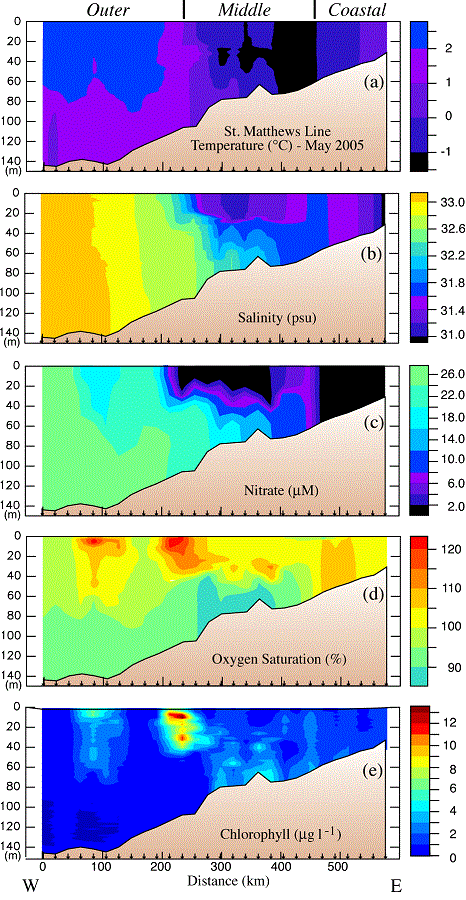
Fig. 9. Hydrographic section along the St. Matthew Island transect during the May 2005 cruise: (a) temperature, (b) salinity, (c) nitrate, (d) percent oxygen saturation and (e) chlorophyll. The y-axes are depth. The domains are indicated at the top of the plot and the locations of specific stations are indicated at the bottom of each panel. Nitrate was measured every ~10 m and at the bottom of each cast.
The middle shelf had a well-defined two-layer structure in salinity and nutrients, but not in temperature (top panel, Fig. 9). The temperature of the shallower portion of the middle domain was colder ( 1°C) than the coastal domain. Oxygen was supersaturated in the surface layer, while nutrients were largely depleted there. In the bottom layer over the middle shelf, lower concentrations of oxygen coincided with an area of slightly elevated chlorophyll. This is consistent with a bloom having already occurred in the surface layer, with portions falling to the benthos. The bottom layer retained significant concentrations of nitrate. In the surface, there was a band of higher nitrate concentrations (6–10 μM) between the depleted waters of the coastal and middle shelf domains (the inner front). This is consistent with observations made farther south at the inner front during previous summers (Kachel et al., 2002). In this frontal region of relatively weak vertical stratification and strong tidal mixing, nutrients from the bottom layer of the middle shelf were mixed upward into the euphotic zone. These processes can result in intermittent production throughout the summer along of the inner front (Jahncke et al., 2005).
The outer domain was characterized by weaker thermal stratification, higher salinity, and slightly warmer temperatures. There were two maxima in chlorophyll: the highest chlorophyll was associated with the offshore edge of the surface, nitrate-depleted zone, a second area of elevated chlorophyll was farther offshore in 140 m of water. Both of these patches of high chlorophyll were associated with water that was supersaturated in dissolved oxygen and slightly reduced nitrate concentrations, indicative of on-going new production.
The daily wind speeds from the NCEP/NCAR Reanalysis during spring–fall calculated at M2 and M8 were significantly correlated (R2 = 0.35), with similar speeds ranging from 0 to 25 m s−1 (Fig. 10). In late May, there was one intense storm (maximum wind velocity >20 m s−1). Summer winds were relatively weak until August when the atmospheric transition to fall conditions began and a series of strong storms began buffeting the region, mixing the water column.
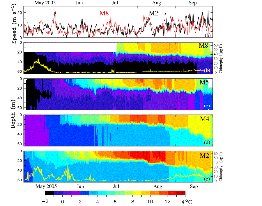
Fig. 10. Time series of wind speed and water temperature during 2005. (a) NCEP wind speed at M2 (black) and M8 (red), (b) through (e) contours of water temperatures at M8, M5, M4, and M2, respectively. The yellow lines at M2 and M8 are the estimates of chlorophyll concentration (μg l−1) derived from the fluorometers. The time period shown is May 1 through September 30, 2005.
While the winds do not vary greatly from north to south, tidal forcing does (Table 1). The two dominant tidal constituents on the eastern Bering Sea shelf are M2 and K1. For the semi-diurnal M2, the amplitudes of the tidal ellipses at the three southern mooring sites (M2, M4, and M5) are similar; however, the amplitude decreased by almost half at M8. In contrast, the amplitude of the diurnal K1 decreases steadily from south to north. Thus, there is significantly less tidal mixing energy at M8 than at M2 or M4. These differences in tidal energy are important to the vertical structure of the water column and are largely invariant on annual and longer timescales.
During spring and summer of the 4-year period, 2004–2007, the mean currents were weak (Table 1), and the velocities were similar to those measured for longer periods at M2 (12–13 years) and M4 (9–10 years). The only location where mean spring-summer currents exceeded 1 cm s−1 was at M5 where there was a westward flow of ~1.5 cm s−1 (Table 1).
In 2005, the general flow, as determined from satellite-tracked drifters, was similar to the schematic of mean currents (Fig. 1). There was a bifurcation of flow at the head of Bering Canyon that left M2 largely isolated from the outer and coastal domains. The flow along the 100-m isobath was weak, but persisted to 60°N, where the flow separated from the 100-m isobath and continued on a northward trajectory toward M8 and into the middle shelf domain (Fig. 1). Unfortunately, no current data were obtained from the ADCPs at M4 and M5 in May–September 2005, but data were collected at M2 and M8 (Table 2). In 2005, the mean currents at M8, while weak, were still stronger than those at M2. Also during 2005, the spring-summer mean speeds at both M2 and M4 (Table 2) were much greater than in the 4-year averages (Table 1). At M8, the average flow during the last several summers has been northward, which differs from the eastward flow (Table 2) that was measured in 2005. The vertical structure in currents was more barotropic at the southern mooring (Δv = −0.2 cm s−1) than at the three moorings farther north (Δv = 0.8–1.2 cm s−1).
While the two southern moorings (M2, M4) were ice free in 2005, the two northern moorings (M5, M8) had ice in their vicinity until early May, and the ice-derived cold pool (bottom temperatures 2°C) which was present most of the summer was limited to the northern shelf (Fig. 10). The warming of the surface waters began in May at all four sites with the two-layer structure evident by June at the three southern moorings and appearing slightly later at M8 (although the upper instrument was at 18 m, so a shallow mixed layer would not have been detected). The water column at M2 and M4 was sharply stratified into upper warm and lower cool layers, while the water column at M5 and M8 had more gradual change between the upper and bottom mixed layers (Fig. 10). As expected, the warmest maximum temperature (>13°C) was at M2, while the coolest was at M8 (<11°C). At all four locations, it appeared that the mixed-layer depth gradually increased after July, with increasing wind strength, thus injecting nitrate into the euphotic zone during the late summer (Fig. 10).
Unfortunately, only two of the fluorometers on the moorings successfully collected data—one at M2 and the other at M8. The spring bloom occurred at both stations in May (Fig. 10). At M8, however, the decrease in chlorophyll after the spring bloom took much longer than at M2; while at M2 there were several events of increased chlorophyll during May and June which resulted from storms (discussed in Section 3.4.3). The chlorophyll temporarily increased at M8 in mid-July (just before the mooring was recovered and redeployed), presumably in response to a storm (Fig. 10a). The water column response to this storm may have been greater at M8 than at M2 because this storm was stronger over the northern shelf than the southern shelf and/or because of less intense stratification at M8 (Fig. 6). It is not known to what extent grazing influenced the decline in chlorophyll, since the relative grazing pressure at each location was unknown. Both M2 and M8 showed a general increase in chlorophyll in late August and September with the increase of storm activity and thus entrainment of nutrients into the surface layer. It must be noted that the fluorescence times series do not provide a comparison of phytoplankton production, but rather an indication of timing and duration of the bloom.
To examine the coupling between wind mixing and increased chlorophyll, we used time series of atmospheric variables (air temperature, total radiation, and the cube of the friction velocity, u*3 – (an indication of wind mixing), ocean temperature, nitrate concentration (at 13 m), and chlorophyll (at 11 m) during a ~40-day period (1 May–9 June; Fig. 11). All variables were measured by instruments on the moorings at M2, including the wind velocity. Since the mean flow at M2 is weak, this is a good location to examine local forcing.
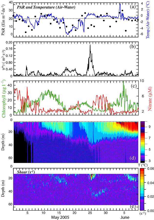
Fig. 11. Time series of atmospheric and oceanographic data from M2 during the month of May. (a) PAR measured at 3 m on the tower of buoy and (air temperature) − (surface water temperature). (b) The friction velocity (u*3) from the hourly winds measured at the buoy. Wind stress was calculated using Large and Pond (1981). (c) chlorophyll at 11 m and the nitrate at 13 m. (d) Temperature was measured at every ~3–4 m and the hourly data were contoured to show temperature structure. (e) Shear measured by a nearby ADCP.
On May 1, the water column was weakly stratified and nutrient concentrations were lower than usual before the spring phytoplankton bloom (historically 16–20 μM; Stabeno et al., 2002). So the 8 μM of nitrate observed on the southern shelf on 1 May was likely an indication of earlier phytoplankton production. During the next 40 days, there were three occasions when chlorophyll increased. These were each associated with a wind event: (1) a 2-day period of weak winds (4–5 May); (2) a 6-day period of stronger winds (17–23 May); and (3) a 4-day period of strong winds (26–29 May).
While the water column was weakly stratified on 1 May, the daily-average solar radiation was >20 Einsteins m−2 d−1. The surface warmed until the first wind event on 4–5 May. There was significant nitrate in the upper water column on 1 May, which was being depleted by the onset of the phytoplankton bloom. On the date of the first storm, there was deepening of the surface mixed layer that introduced more nitrate into the surface layer. Nitrate values decreased to near 2 μM on ~8 May, with the chlorophyll peaking on 11 May (~7 days after the onset of the first storm).
The temperature in the upper 25 m continued to increase until 17 May, when the period (17–21 May) of low, but sustained wind stress and cooling of the ocean surface eroded the stratification and injected nitrate upward into the surface layer. This second mixing event was associated with a period of reduced total radiation and cold air temperatures that cooled the upper water column (Fig. 11d), thus reducing stratification and permitting greater deepening of the surface mixed layer. Nitrate concentration began increasing on 18 May. Chlorophyll began to increase about the same time and reached a maximum around 23 May (6 days after the onset of the storm).
As the third and most energetic storm mixed the water column to 50 m, surface nitrate rapidly increased from near zero to >6 μM and remained at that concentration for about 4 days. Active mixing of the water column is evident in the shear to a depth of ~50 m (Fig. 11e). The chlorophyll slowly increased to a maximum on 5 June. Temperature in the upper 5 m of the water column, which had begun to increase soon after the third storm passed, reached a maximum just before the maximum in chlorophyll. The lag from storm initiation to maximum nitrate was about 4 days; the lag between storm initiation and an increase in chlorophyll was 6 or 7 days; and it was 12 days between storm initiation and the maximum chlorophyll. During this third "spring bloom," chlorophyll continued to increase after the concentrations of nitrate were reduced.
The lag between the beginning of the storms and maximum chlorophyll was ~6 days for the weaker storms and 12 days for the stronger storm. These observed lag times between storm, nutrient input, and phytoplankton blooms may be of interest to those attempting to model lower trophic level dynamics. With continued monitoring we may be able to improve parameterization of numerical simulations of the timing among storms, mixing, and phytoplankton blooms (i.e., coupled physics-NPZ models). This will result in a better understanding of the processes that control not only the spring phytoplankton bloom, but summer production as well (Sambrotto et al., 1986). Variation in the solar radiation, strength of the storm, phytoplankton compensation depth, microzooplankton grazing pressure, and the species of phytoplankton that comprised the bloom could all have contributed to differences in the lag times between the storms and the phytoplankton blooms.
The influence of winds on the ocean is dependent upon water column stratification. This was evident at M2 on 5 May, when a relatively weak storm mixed the water column and introduced substantial amounts of nitrate into the euphotic zone. Stratification subsequently increased at M2 and the following storm was less successful at replenishing the nitrate despite a longer period of significant winds. Differences in stratification at M2 and M8 could impact the phytoplankton blooms at the two locations. For instance, the third storm (26–29 May) was also evident in the modeled winds from the NCEP Reanalysis (Fig. 10a) at both M2 (black) and M8 (red). In response to this storm, there was an increase in chlorophyll at M2, but not at M8. The different chlorophyll concentrations may be due, in part, to differences in stratification. The spring bloom occurred at about the same time at each location, but the chlorophyll time series at M8 showed a single relatively long event, while the chlorophyll time series at M2 showed three relatively shorter events. This is something that we may not have predicted given the data and initial paradigm offered for the spring bloom at site M2 (Hunt et al., 2002; Stabeno and Hunt, 2002).
The temperature/salinity (T–S) patterns obtained from time series of temperature and salinity measured on the moorings (May–September) were distinctly different among the two southern, the central, and the northern mooring sites (Fig. 12). Data from three different depths from the two southern moorings (M2, M4) show seasonal warming with a slight decrease in salinity over the course of the summer. Thus the density at all depths decreased during the time period. This is consistent with previous observations at M2 (Stabeno et al., 2007). In sharp contrast, data from the central (M5) and the northern moorings (M8) show considerable (~1 psu), variability in the salinity. At these moorings, the near-bottom salinity increased over the deployment period and although there was some warming the density increased during the summer months. The near-surface salinity was highly variable, especially in July–August, where short periods (~week long) of lower or higher salinity occur. These are likely the result of advection. The near surface water became less dense during the summer.
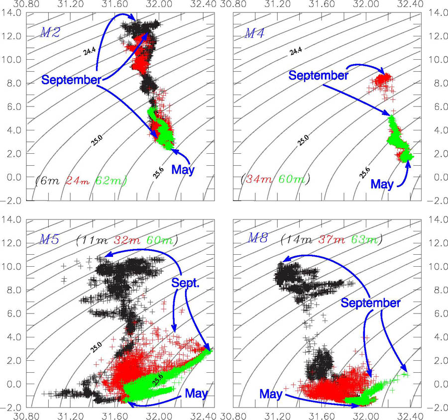
Fig. 12. Hourly temperature and salinity data from each moorings from three depths: near surface (black), mid-water (red), and near bottom (green). These panels show how the temperature and salinity changed over the course of the deployment (May to September). The near-surface instrument at M4 failed, so there are only two time series in that panel. The beginning of the time series (May) is indicated and the middle September is also indicated.
In May, at the beginning of the time series, the water at M5 and M8 was fresher than at M2 and M4, as a result of ice melt and the vertical mixing of this fresher water throughout the water column. Immediately after the water column became stratified, the temperature remained <−1°C at M5, but the surface freshened by ~0.6 psu, while the deeper water became more saline by ~0.4 psu. Ice persisted to the east and north of St. Matthew Island into June. As seen in the historical currents (Table 2), the flow at M5 is westward. Hence, the melting of ice behind St. Matthew would result in fresher surface water during late spring, which could then be advected past the mooring. By September the bottom salinity at M5 had increased to a concentration similar to that observed at M4 at the beginning of May.
At M8 there appeared to be periods of increased salinity in the surface waters. This occurred in mid to late summer, and the source is likely water that was advected northward along the 100-m isobath and then onto the middle shelf as seen in the trajectories of satellite-tracked drifters (Fig. 1). As the summer progressed the bottom instrument at M8 showed an increase of salinity accompanied by a slight warming. This increase in salinity at M8 was not as substantial as that observed at M5.
Cross shelf and along shelf advection were the cause of the temporal changes in salinity at the moorings. At M2 and M4 the changes were relatively small, since advection at these two moorings was weak during the summer (Stabeno et al., 2007). At M5 and M8, however, the near-bottom increase in salinity after June indicated the importance of advection at these locations. One distinct possible source of water is the Pribilof region, where bottom salinities (60–100 m water depth) range from 32.0 to 32.6 (Stabeno et al., 2007). Historically, drifter trajectories have revealed a weak on-shelf flow somewhere between M4 and M5 (Flint et al., 2002; Stabeno et al., 2006); this cross-shelf flow originates just north of the Pribilof Islands. Evidence for a cross-shelf flux was also found in changes in the spatial extent of the cold pool. A cold pool forms over that portion of the shelf, and as summer progresses this southern cold pool often becomes isolated from the northern cold pool, with warmer temperatures occurring somewhere between M4 and M5 (Wyllie-Echeverria, 1995a,b).
Historical reports of the broad-scale distribution of Bering Sea zooplankton communities also support the hypothesis that cross shelf advection of species occurs regularly on the shelf (e.g., Vinogradov, 1956; Motoda and Minoda, 1974). Zooplankton community distribution maps from the Russian literature describe an intrusion of oceanic organisms into the middle shelf domain north of the Pribilof Islands, inshore to about the latitude of Nunivak Island (Cooney, 1981; Coyle et al., 1996). The location of this intrusion is very similar to where we found the North–South Transition that was formed after the advection of slope or outer shelf water occupied the middle shelf. Similarly, Coyle and Pinchuk (2002b) detected oceanic and outer domain species near the inner front (ca. 50 m isobath) in this region. However, neither our spring nor late summer 2005 samples in that area showed significant concentrations of oceanic community species such as Neocalanus spp., Eucalanus bungii, or Metridia pacifica. The spring densities of these taxa (1–5 m−3) were greater farther south, between CTD Stations 94 and 118, perhaps due to on-shelf transport at Bering Canyon or transport across the shelf during spring before the frontal structure had become established.
These physical and biological observations support the hypothesis that the source of the warmer, more saline water observed at M5 and to a lesser extent at M8 was the outer shelf in the vicinity of the Pribilof Islands. The exact pathway is unknown. One possibility (supported by historical data) is that the weak onshelf flow north of St. Paul Island introduces water from the vicinity of the Pribilof Islands onto the shelf south of M5.
During 2005, the modeled winds did not differ significantly between the northern and southern shelves. Water-column stratification varied from north to south with a sharp two-layer structure over the southern middle shelf and more gradual vertical density gradient over the northern middle shelf (Fig. 6). This was largely due to the decrease in tidal mixing energy with increasing latitude. In the spring, the vertical structure of the northern shelf is weakly stratified by temperature and moderately stratified by salinity. By early autumn, the southern shelf is stratified almost completely by temperature and the northern shelf by a combination of temperature and salinity. Following Carmack (2007), there is a temptation to refer to the salinity influenced northern portion of the Bering shelf as a beta ocean and the temperature-dominated southern portion as an alpha ocean, but such a designation would not be appropriate for this region. Carmack (2007) described the ocean basins, where such a differentiation is long lasting. In contrast the salinity-temperature structure on the shelf can be ephemeral and dependent upon the year-to-year variability in sea-ice extent.
The presence/absence of sea ice modifies the physics, chemistry, and biology of the Bering Sea shelf. In the spring, the northern limit of the southern shelf was determined by the southern extent of spring ice. Advection modified the position of the transition zone between the north and south over the middle shelf. In 2005, this resulted in a northward shift of the transition between the northern and southern shelves during late spring and early summer. Other than the position of this transition zone, differences between the north and southern middle shelf, that were set up by ice, persisted through summer. Whether this occurs each year is not known, although we would hypothesize that in other years sea ice would influence the structure over the shelf and a northward shift would occur, since the weak flow patterns over this shelf appear to be consistent from year to year (Stabeno et al., 2007). The position of the cross-shelf flow that occurs north of the Pribilof Islands, however, may change from year to year, since it is probably related to the baroclinic structure over the shelf. This structure is dependent upon maximum ice extent, so this boundary between the northern and southern shelves will vary because of variability in the spatial position and timing of maximum ice extent. It must be noted that climate models predict that the maximum ice extent over the eastern Bering Sea shelf will remain south of St. Matthew Island. Thus the division between the northern shelf and southern shelf, as evidenced by the extent of the cold pool, will likely remain in the vicinity of St. Matthew Island.
In contrast to the stability of the middle domain, water properties resulting from presence of sea ice over the outer shelf did not persist. Flow over the outer shelf (particularly along the 100-m isobath, Fig. 1) is stronger than over the middle domain. In addition, the outer shelf interacts with water from the slope and basin. In particular, instabilities over the slope can result in intrusions of slope water onto the shelf (Stabeno and van Meurs, 1999; Schumacher and Stabeno, 1998; Mizobata et al., 2008). All these can modify the water properties over the outer shelf.
There was a significant reduction (~50%) in nitrate concentrations on the northern shelf during the summer that was likely a result of nutrient uptake by phytoplankton. In addition, there were unprecedented nitrite concentrations in the summer in an area that had been covered by ice and modified through advection. These high concentrations were perhaps a result of uncoupled nitrification.
During spring, the zooplankton communities differed between the northern and southern middle shelf domains. In late summer 2005, biological processes may have acted to erase differences in zooplankton community structure created by the initial conditions during winter and spring.
The work presented here significantly increases our understanding of the patterns and processes over the eastern Bering Sea shelf and complements the focused studies of the Bering Strait region between St. Lawrence Island and Bering Strait (Grebmeier, 1993) and the examinations of how ice influences these ecosystems (Clement et al., 2004, 2005). Historically, northern and southern regions of the Bering Sea shelf have been defined by absolute geographic coordinates, but from an ecosystem perspective, north and south may be more appropriately defined by a physical, chemical, and biological structure that is a response to the presence or absence of seasonal sea ice. In spring 2005, the transition between the northern and southern shelves was evident in the temperature, salinity, vertical density structure (Brunt-Väisälä frequency), surface nutrients, and the zooplankton community (Figs. 4 and 8), while in late summer, it was most evident in the surface salinity, bottom temperatures, and surface nutrients (Fig. 5).
In 2005, the southern shelf ice-free area stretched from the Alaska Peninsula to approximately Station 91, while the transition region extended from Station 91 to just south of St. Matthew Island. The northern portion of the middle shelf stretched from the northern end of the transition to St. Lawrence Island where the middle shelf ends. So, in addition to the standard cross-shelf domains (coastal, middle, and outer), there are, at least over the middle shelf, a northern domain and a southern domain. We suggest the southern part of the middle shelf retain the name of the Middle Shelf Domain, while the northern part be called the Northern Middle Shelf Domain with the transition between them identified as the North-South Transition.
The results reported here are from a single year, 2005, with limited ice extent. They are the patterns one would expect in the early stages of a warming cycle. Results from low, moderate, and high ice years are necessary to understand if the observations and mechanisms proposed here are valid for the full range of ecosystem response. At the time of this writing we are in a period of extensive ice, and cool to extreme cold for the eastern Bering Sea. Two new programs, the Bering Ecosystem Study (BEST) and the Bering Sea Integrated Ecosystem Research Program (BSIERP) are providing the data to examine our conclusions.
Acknowledgments. We thank D. Kachel and N. Kachel for data analysis and S. Salo for providing satellite images. S. Salo, D. Kachel, P. Proctor, A. Jenkins, J. Clark, K. Mier, R. Cartwright, W. Floering, C. DeWitt, D. Righi, M. Dunlap, S. Smith, S. Thornton, and B. Munger provided assistance at sea and were responsible for collecting the majority of our data. C. Harpold provided assistance with chlorophyll sample analyses, and chlorophyll and zooplankton data management. We thank K. Coyle and G.L. Hunt Jr. for their comments on an early draft of this paper. K. Birchfield and K. McKinney provided graphics work and R.L. Whitney did the technical editing. We thank the officers and crews of the NOAA ship Miller Freeman and R/V Thomas G. Thompson for invaluable assistance in making these oceanographic measurements. This research was funded by NOAA's North Pacific Climate Regimes and Ecosystem Productivity Program and the North Pacific Research Board (Grants: #517, 602, 701). This is contribution FOCI-N688 to the Ecosystems and Fisheries Oceanography Coordinated Investigations; 1813 to Joint Institute for the Study of the Atmosphere and Ocean, University of Washington, and 3197 to PMEL.
Baier, C. T., and J. M. Napp, 2003. Climate-induced variability in Calanus marshallae populations. Journal of Plankton Research, 25, 771–782.
Baier, C. T., and M. Terazaki, 2005. Interannual variability in a predator-prey interaction: Climate, chaetognaths and copepods in the Southeastern Bering Sea. Journal of Plankton Research, 27, 1113–1125.
Bailey, K. M., E. S. Brown, and J. T. Duffy-Anderson, 2003. Aspects of distribution, transport and recruitment of Alaska plaice (Pleuronectes quadrituberculatus) in the Gulf of Alaska and eastern Bering Sea: comparison of marginal and central populations. Journal of Sea Research, 50, 87–95.
Bond, N. A., and J. M. Adams, 2002. Atmospheric forcing of the southeast Bering Sea Shelf during 1995–99 in the context of a 40-year historical record. Deep-Sea Research II, 49(26), 5869–5887.
Carmack, E., 2007. The alpha/beta ocean distinction: a perspective on freshwater fluxes, ventilation, nutrients and primary productivity in high-latitude seas. Deep-Sea Research II, 54, 2578–2598. doi:10.1016/j.dsr2.2007.08.018.
Ciannelli, L., and K. M. Bailey, 2005. Landscape dynamics and resulting species interactions: the cod-capelin system in the southeastern Bering Sea. Marine Ecology Progress Series, 291, 227–236.
Clement, J. L., L. W. Cooper, and J. M. Grebmeier, 2004. Late-winter water column and sea ice conditions in the northern Bering Sea. Journal of Geophysical Research, 109. doi:10.1029/2003JC002047.
Clement, J. L., W. Maslowski, L. W. Cooper, J. M. Grebmeier, and W. Walczowski, 2005. Ocean circulation and exchanges through the northern Bering Sea: 1979–2001 model results. Deep-Sea Research II, 52, 3509–3540.
Coachman, L. K., 1986. Circulation, water masses and fluxes on the southeastern Bering Sea shelf. Continental Shelf Research, 5, 23–108.
Cooney, R. T., 1981. Bering Sea zooplankton and micronekton communities with emphasis on annual production. In: Hood, D. W., Calder, J. A. (Eds.), The Eastern Bering Sea Shelf: Oceanography and Resources, NOAA Office of Marine Pollution Assessment, vol. 2. University of Washington Press, pp. 947–974.
Cooney, R. T., and K. O. Coyle, 1982. Trophic implications of cross-shelf copepod distributions in the southeastern Bering Sea. Marine Biology, 70, 187–196.
Coyle, K. O., and A. I. Pinchuk, 2002a. Climate-related differences in zooplankton density and growth on the inner shelf of the southeastern Bering Sea. Progress in Oceanography, 55, 177–194.
Coyle, K. O., and A. I. Pinchuk, 2002b. The abundance and distribution of euphausiids and zero-age pollock on the inner shelf of the southeast Bering Sea near the Inner Front in 1997–1999. Deep-Sea Research Part II, 49, 6009–6030.
Coyle, K. O., V. G. Chavtur, and A. I. Pinchuk, 1996. Zooplankton of the Bering Sea: A review of the Russian-language literature. In: Mathisen, O. A., and Coyle, K. O. (Eds.), Ecology of the Bering Sea: A Review of the Russian Literature. Alaska Sea Grant College Program Report No. 96-01, University of Alaska, Fairbanks, pp. 97–133.
Coyle, K. O., A. I. Pinchuk, L. B. Eisner, and J. M. Napp, 2008. Zooplankton species composition, abundance and biomass on the eastern Bering Sea shelf during summer: The potential role of water column stability and nutrients in structuring the zooplankton community. Deep-Sea Research II, 55, 1775–1791.
Flint, M. V., I. N. Sukhanova, A. I. Kopylov, S. G. Poyarkov, and T. E. Whitledge, 2002. Plankton distribution associated with frontal zones in the vicinity of the Pribilof Islands. Deep-Sea Research II, 49, 6069–6093.
Frost, B. R., 1974. Calanus marshallae, a new species of calanoid copepod closely allied to the sibling species of C. Finmarchicus and C. glacialis. Marine Biology, 26, 77–99.
Gordon, L. I., J. C. Jennings, Jr., A. A. Ross, and J. M. Krest, 1993. A suggested protocol for continuous automated analysis of seawater nutrients (phosphate, nitrate, nitrite and silicic acid) in the WOCE Hydrographic program and the Joint Global Ocean Fluxes Study. WOCE Operations Manual, vol. 3: The Observational Programme, Section 3.2: WOCE Hydrographic Programme, Part 3.1.3: WHP Operations and Methods. WHP Office Report WHPO 91-1; WOCE Report No. 68/91. November 1994, Revision 1, Woods Hole, MA, USA, 52 loose-leaf pages.
Grebmeier, J. M., 1993. Studies of pelagic-benthic coupling extended onto the Soviet continental shelf in the Bering and Chukchi Seas. Continental Shelf Research, 13, 653–666.
Grebmeier, J. M., and J. P. Barry, 2007. Benthic processes in polynyas. In Smith Jr., W. O., and D. G. Barber (Eds.) Polynyas: Windows to the World, Elsevier Oceanography Series, vol. 74, pp. 363–390.
Grebmeier, J. M., and K. H. Dunton, 2000. Benthic processes in the Northern Bering/Chukchi Seas: Status and global change. In Huntington, H. P. (Ed.), Impacts of Changes in Sea Ice and Other Environmental Parameters in the Arctic. Marine Mammal Commission Workshop, Girdwood, Alaska, 15–17 February 2000, pp. 80–93.
Grebmeier, J. M., J. E. Overland, S. E. Moore, E. V. Farley, E. C. Carmack, L. W. Cooper, K. E. Frey, J. H. Helle, F. A. McLaughlin, and S. L. McNutt, 2006. A major ecosystem shift in the northern Bering Sea. Science, 311, 1461–1464.
Hunt, Jr., G. L., and K. F. Drinkwater, 2005. Ecosystem studies of Sub-Arctic Seas (ESSAS) Science Plan. GLOBEC Report No. 19, 600 pp.
Hunt, Jr., G. L., P. J. Stabeno, G. Walters, E. Sinclair, R. D. Brodeur, J. M. Napp, and N. A. Bond, 2002. Climate change and control of the southeastern Bering Sea pelagic ecosystem. Deep Sea Research Part II, 49, 5821–5853.
Hunt, Jr., G. L., P. J. Stabeno, S. Strom, and J. M. Napp, 2008. Patterns of spatial and temporal variation in the marine ecosystem of the southeastern Bering Sea, with special reference to the Pribilof Domain. Deep-Sea Research II, 55, 1919–1944.
IPCC, 2007. Climate Change 2007: The physical science basis. Intergovernmental Panel on Climate Change, Geneva, Switzerland.
Jahncke, J., K. O. Coyle, S. I. Zeeman, N. B. Kachel, and G. L. Hunt, Jr., 2005. Distribution of foraging shearwaters relative to the inner front of the SE Bering Sea. Marine Ecological Progress Series, 305, 219–233.
Kachel, N. B., G. L. Hunt, Jr., S. A. Salo, J. D. Schumacher, P. J. Stabeno, and T. E. Whitledge, 2002. Characteristics and variability of the inner front of the southeastern Bering Sea. Deep-Sea Research II, 49, 5889–5909.
Kalnay, E., M. Kanamitsu, R. Kistler, W. Collins, D. Deaven, L. Gandin, M. Iredell, S. Saha, G. White, J. Woollen, Y. Zhu, A. Leetmaa, B. Reynolds, M. Chelliah, W. Ebisuzaki, W. Higgins, J. Janowiak, K. Mo, C. Ropelewski, J. Wang, R. Jenne, and D. Joseph, 1996. The NCEP/NCAR 40-year reanalysis project. Bulletin of the American Meteorological Society, 77, 437–471.
Ladd, C., and N. A. Bond, 2002. Evaluation of the NCEP-NCAR Reanalysis in the northeast Pacific and Bering Sea. Journal of Geophysical Research, 107, 3158. doi:10.1029/2001JC001157.
Large, W. G., and S. Pond, 1981. Open ocean momentum flux measurements in moderate to strong winds. Journal of Physical Oceanography, 11, 324–336.
Lovvorn, J. R., S. E. Richman, J. M. Grebmeier, and L. W. Cooper, 2003. Diet and body condition of spectacled eiders in pack ice of the Bering Sea. Polar Biology, 26, 259–267.
Mizobata, K., S.-I. Saitoh, and J. Wang, 2008. Interannual variability of summer biochemical enhancement in relation to mesoscale eddies at the shelf break in the vicinity of the Pribilof Islands, Bering Sea. Deep-Sea Research II, 55, 1717–1728.
Mordy, C. W., P. J. Stabeno, D. Righi, and F. A. Menzia, 2008. Origins of the sub-surface ammonium maximum in the southeast Bering Sea. Deep Sea Research II, 55, 1738–1744.
Motoda, S., and T. Minoda, 1974. Plankton of the Bering Sea. In Hood, D. W., and E. J. Kelley (Eds.) Oceanography of the Bering Sea, Institute of Marine Science Occasional Publication No. 2. University of Alaska, Fairbanks, pp. 207–410.
Niebauer, H. J., N. A. Bond, L. P. Yakunin, and V. V. Plotnikov, 1999. An update on the climatology and sea ice in the Bering Sea. In Loughlin, T. R., and K. Ohtani (Eds.) Dynamics of the Bering Sea. University of Alaska Sea Grant Program, AK-SG-03, Fairbanks, pp. 29–59, 838 pp.
Overland, J. E., and P. J. Stabeno, 2004. Is the climate of the Bering Sea warming and affecting the ecosystem? Eos Transactions of the American Geophysical Union, 85, 309–316.
Peterson, W. T., C. B. Miller, and A. Hutchinson, 1979. Zonation and maintenance of copepod populations in the Oregon upwelling zone. Deep-Sea Research, 26, 467–494.
Rho, T. K., T. E. Whitledge, and J. J. Goering, 2005. Interannual variations of nutrients and primary production over the Southeastern Bering Sea Shelf during the spring of 1997, 1998, and 1999. Oceanology, 45, 376–390.
Sambrotto, R. N., H. J. Niebauer, J. J. Goering, and R. L. Iverson, 1986. Relationships among vertical mixing, nitrate uptake and phytoplankton growth during the spring bloom in the southeast Bering Sea middle shelf. Continental Shelf Research, 5, 161–198.
Schneider, D. C., G. L. Hunt, Jr., and N. M. Harrison, 1986. Mass and energy transfer to seabirds in the southeastern Bering Sea. Continental Shelf Research, 5, 241–257.
Shumacher, J. D., and P. J. Stabeno, 1998. Continental shelf of the Bering Sea. In A. R. Robinson and K. H. Brink (Eds.), The Sea, vol. 11. John Wiley and Sons, pp. 789–822 (Chapter 27).
Sirenko, B. I., and V. M. Koltun, 1992. Characteristics of benthic biocenoses of the Chukchi and Bering seas. In P. A. Nagel (Ed.), Results of the Third Joint US-USSR Bering and Chukchi Seas Expedition (BERPAC). Summer 1988. US Fish and Wildlife Service, Washington, DC, pp. 251–261.
Smith, S. L., 1991. Growth, development and distribution of the euphausiids Thysanoessa raschi (M. Sars) and Thysanoessa inermis (Kroyer) in the southeastern Bering Sea. Polar Research, 10, 461–478.
Smith, S.L., and J. Vidal, 1986. Variations in the distribution abundance, and development of copepods in the southeastern Bering Sea in 1980 and 1981. Continental Shelf Research 5, 215–239.
Springer, A. M., C. P. McRoy, and M. V. Flint, 1996. The Bering Sea Green Belt: shelf-edge processes and ecosystem production. Fisheries Oceanography 5, 205–223.
Stabeno, P. J., and G. L. Hunt, Jr., 2002. Overview of the inner front and southeast Bering Sea carrying capacity programs. Deep-Sea Research II 49(26), 6157–6168.
Stabeno, P. J., and P. van Meurs, 1999. Evidence of episodic on-shelf flow in the southeastern Bering Sea. Journal of Geophysical Research 104 (29), 715–729.
Stabeno, P. J., N. B. Kachel, M. Sullivan, and T. E. Whitledge, 2002. Variability of physical and chemical characteristics along the 70-m isobath of the southeast Bering Sea. Deep-Sea Research Part II 49, 5931–5943.
Stabeno, P. J., G. L. Hunt, Jr., J. M. Napp, and J. D. Schumacher, 2006. Physical forcing of ecosystem dynamics on the Bering Sea shelf. In: Robinson, A.R. Brink, K.H. (Eds.), The Sea, vol. 14, pp. 1177–1212.
Stabeno, P. J., N. A. Bond, N. B. Kachel, and S. A. Salo, 2007. On the recent warming of the Southeastern Bering Sea Shelf. Deep-Sea Research II 54, 2599–2618.
Sullivan, M. E., N. B. Kachel, C. W. Mordy, and P. J. Stabeno, 2008. The Pribilof Islands: temperature, salinity and nitrate during summer 2004. Deep-Sea Research Part II 55, 1729–1737.
Vinogradov, M. E., 1956. Zooplankton distribution in the western Bering Sea. Tr. Vses. Gidrobiol. Ova. (Translation All-Union Hydrobiological Society) 7, 173–203 (in Russian).
Walsh, J. J., and C. P. McRoy, 1986. Ecosystem analysis in the southeastern Bering Sea. Continental Shelf Research 5, 259–288.
Whitledge, T. E., W. S. Reeburgh, and J. J. Walsh, 1986. Seasonal inorganic nitrogen distributions and dynamics in the southeastern Bering Sea. Continental Shelf Research 5, 109–132.
Wyllie-Echeverria, T., 1995a. Sea–ice conditions and the distribution of walleye pollock (Theragra chalcogramma) on the Bering and Chukchi Sea shelf. In: Beamish, R.J. (Ed.), Climate Change and Northern Fish Populations, Canadian Special Publication of Fisheries and Aquatic Sciences 121, pp. 131–136.
Wyllie-Echeverria, T., 1995b. Seasonal sea ice, the cold pool and gadid distribution on the Bering Sea shelf. Ph.D. Dissertation, Univ. Alaska, Fairbanks, 281 pp.
Wyllie-Echeverria, T., and K. Ohtani, 1999. Seasonal sea ice variability and the Bering Sea ecosystem. In: T. R. Loughlin and K. Ohtani (Eds.), Dynamics of the Bering Sea. University of Alaska Sea Grant, AK-SG-03, Fairbanks, pp. 435–451, 838 pp.
Go to Abstract