The daily wind speeds from the NCEP/NCAR Reanalysis during spring–fall calculated at M2 and M8 were significantly correlated (R2 = 0.35), with similar speeds ranging from 0 to 25 m s−1 (Fig. 10). In late May, there was one intense storm (maximum wind velocity >20 m s−1). Summer winds were relatively weak until August when the atmospheric transition to fall conditions began and a series of strong storms began buffeting the region, mixing the water column.
Fig. 10. Time series of wind speed and water temperature during 2005. (a) NCEP wind speed at M2 (black) and M8 (red), (b) through (e) contours of water temperatures at M8, M5, M4, and M2, respectively. The yellow lines at M2 and M8 are the estimates of chlorophyll concentration (μg l−1) derived from the fluorometers. The time period shown is May 1 through September 30, 2005.
While the winds do not vary greatly from north to south, tidal forcing does (Table 1). The two dominant tidal constituents on the eastern Bering Sea shelf are M2 and K1. For the semi-diurnal M2, the amplitudes of the tidal ellipses at the three southern mooring sites (M2, M4, and M5) are similar; however, the amplitude decreased by almost half at M8. In contrast, the amplitude of the diurnal K1 decreases steadily from south to north. Thus, there is significantly less tidal mixing energy at M8 than at M2 or M4. These differences in tidal energy are important to the vertical structure of the water column and are largely invariant on annual and longer timescales.
Table 1. The mean water velocity during 1 April–30 September. All the sites were instrumented from 2004 to 2007. In addition, data were collected during 1995–2007 for M2 and for 1997–2007 for M4. For each site, the April–May averages were calculated for the four years (2004–2007) and for M2 and M4, averages were also calculated for total record. The number of years is indicated in the third column and the total number of months of data is indicated in parenthesis. If there was at least one month of data during that period, then that year is listed as having data.
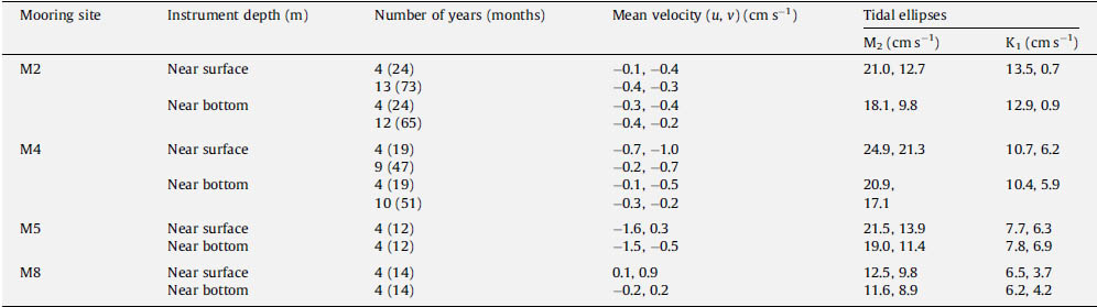
During spring and summer of the 4-year period, 2004–2007, the mean currents were weak (Table 1), and the velocities were similar to those measured for longer periods at M2 (12–13 years) and M4 (9–10 years). The only location where mean spring-summer currents exceeded 1 cm s−1 was at M5 where there was a westward flow of ~1.5 cm s−1 (Table 1).
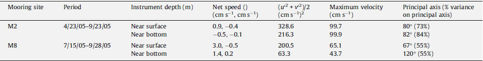
In 2005, the general flow, as determined from satellite-tracked drifters, was similar to the schematic of mean currents (Fig. 1). There was a bifurcation of flow at the head of Bering Canyon that left M2 largely isolated from the outer and coastal domains. The flow along the 100-m isobath was weak, but persisted to 60°N, where the flow separated from the 100-m isobath and continued on a northward trajectory toward M8 and into the middle shelf domain (Fig. 1). Unfortunately, no current data were obtained from the ADCPs at M4 and M5 in May–September 2005, but data were collected at M2 and M8 (Table 2). In 2005, the mean currents at M8, while weak, were still stronger than those at M2. Also during 2005, the spring-summer mean speeds at both M2 and M4 (Table 2) were much greater than in the 4-year averages (Table 1). At M8, the average flow during the last several summers has been northward, which differs from the eastward flow (Table 2) that was measured in 2005. The vertical structure in currents was more barotropic at the southern mooring (Δv = −0.2 cm s−1) than at the three moorings farther north (Δv = 0.8–1.2 cm s−1).
Table 2. Statistics at the northern and southernmost moorings in 2005 (no data were available at M4 and M5). Near surface measurements were at depths 10–20 m and near bottom measurements were at 55–62 m.
While the two southern moorings (M2, M4) were ice free in 2005, the two northern moorings (M5, M8) had ice in their vicinity until early May, and the ice-derived cold pool (bottom temperatures  2°C) which was present most of the summer was limited to the northern shelf (Fig. 10). The warming of the surface waters began in May at all four sites with the two-layer structure evident by June at the three southern moorings and appearing slightly later at M8 (although the upper instrument was at 18 m, so a shallow mixed layer would not have been detected). The water column at M2 and M4 was sharply stratified into upper warm and lower cool layers, while the water column at M5 and M8 had more gradual change between the upper and bottom mixed layers (Fig. 10). As expected, the warmest maximum temperature (>13°C) was at M2, while the coolest was at M8 (<11°C). At all four locations, it appeared that the mixed-layer depth gradually increased after July, with increasing wind strength, thus injecting nitrate into the euphotic zone during the late summer (Fig. 10).
Unfortunately, only two of the fluorometers on the moorings successfully collected data—one at M2 and the other at M8. The spring bloom occurred at both stations in May (Fig. 10). At M8, however, the decrease in chlorophyll after the spring bloom took much longer than at M2; while at M2 there were several events of increased chlorophyll during May and June which resulted from storms (discussed in Section 3.4.3). The chlorophyll temporarily increased at M8 in mid-July (just before the mooring was recovered and redeployed), presumably in response to a storm (Fig. 10a). The water column response to this storm may have been greater at M8 than at M2 because this storm was stronger over the northern shelf than the southern shelf and/or because of less intense stratification at M8 (Fig. 6). It is not known to what extent grazing influenced the decline in chlorophyll, since the relative grazing pressure at each location was unknown. Both M2 and M8 showed a general increase in chlorophyll in late August and September with the increase of storm activity and thus entrainment of nutrients into the surface layer. It must be noted that the fluorescence times series do not provide a comparison of phytoplankton production, but rather an indication of timing and duration of the bloom.
To examine the coupling between wind mixing and increased chlorophyll, we used time series of atmospheric variables (air temperature, total radiation, and the cube of the friction velocity, u*3 – (an indication of wind mixing), ocean temperature, nitrate concentration (at 13 m), and chlorophyll (at 11 m) during a ~40-day period (1 May–9 June; Fig. 11). All variables were measured by instruments on the moorings at M2, including the wind velocity. Since the mean flow at M2 is weak, this is a good location to examine local forcing.
Fig. 11. Time series of atmospheric and oceanographic data from M2 during the month of May. (a) PAR measured at 3 m on the tower of buoy and (air temperature) − (surface water temperature). (b) The friction velocity (u*3) from the hourly winds measured at the buoy. Wind stress was calculated using Large and Pond (1981). (c) chlorophyll at 11 m and the nitrate at 13 m. (d) Temperature was measured at every ~3–4 m and the hourly data were contoured to show temperature structure. (e) Shear measured by a nearby ADCP.
On May 1, the water column was weakly stratified and nutrient concentrations were lower than usual before the spring phytoplankton bloom (historically 16–20 μM; Stabeno et al., 2002). So the 8 μM of nitrate observed on the southern shelf on 1 May was likely an indication of earlier phytoplankton production. During the next 40 days, there were three occasions when chlorophyll increased. These were each associated with a wind event: (1) a 2-day period of weak winds (4–5 May); (2) a 6-day period of stronger winds (17–23 May); and (3) a 4-day period of strong winds (26–29 May).
While the water column was weakly stratified on 1 May, the daily-average solar radiation was >20 Einsteins m−2 d−1. The surface warmed until the first wind event on 4–5 May. There was significant nitrate in the upper water column on 1 May, which was being depleted by the onset of the phytoplankton bloom. On the date of the first storm, there was deepening of the surface mixed layer that introduced more nitrate into the surface layer. Nitrate values decreased to near 2 μM on ~8 May, with the chlorophyll peaking on 11 May (~7 days after the onset of the first storm).
The temperature in the upper 25 m continued to increase until 17 May, when the period (17–21 May) of low, but sustained wind stress and cooling of the ocean surface eroded the stratification and injected nitrate upward into the surface layer. This second mixing event was associated with a period of reduced total radiation and cold air temperatures that cooled the upper water column (Fig. 11d), thus reducing stratification and permitting greater deepening of the surface mixed layer. Nitrate concentration began increasing on 18 May. Chlorophyll began to increase about the same time and reached a maximum around 23 May (6 days after the onset of the storm).
As the third and most energetic storm mixed the water column to 50 m, surface nitrate rapidly increased from near zero to >6 μM and remained at that concentration for about 4 days. Active mixing of the water column is evident in the shear to a depth of ~50 m (Fig. 11e). The chlorophyll slowly increased to a maximum on 5 June. Temperature in the upper 5 m of the water column, which had begun to increase soon after the third storm passed, reached a maximum just before the maximum in chlorophyll. The lag from storm initiation to maximum nitrate was about 4 days; the lag between storm initiation and an increase in chlorophyll was 6 or 7 days; and it was 12 days between storm initiation and the maximum chlorophyll. During this third "spring bloom," chlorophyll continued to increase after the concentrations of nitrate were reduced.
The lag between the beginning of the storms and maximum chlorophyll was ~6 days for the weaker storms and 12 days for the stronger storm. These observed lag times between storm, nutrient input, and phytoplankton blooms may be of interest to those attempting to model lower trophic level dynamics. With continued monitoring we may be able to improve parameterization of numerical simulations of the timing among storms, mixing, and phytoplankton blooms (i.e., coupled physics-NPZ models). This will result in a better understanding of the processes that control not only the spring phytoplankton bloom, but summer production as well (Sambrotto et al., 1986). Variation in the solar radiation, strength of the storm, phytoplankton compensation depth, microzooplankton grazing pressure, and the species of phytoplankton that comprised the bloom could all have contributed to differences in the lag times between the storms and the phytoplankton blooms.
The influence of winds on the ocean is dependent upon water column stratification. This was evident at M2 on 5 May, when a relatively weak storm mixed the water column and introduced substantial amounts of nitrate into the euphotic zone. Stratification subsequently increased at M2 and the following storm was less successful at replenishing the nitrate despite a longer period of significant winds. Differences in stratification at M2 and M8 could impact the phytoplankton blooms at the two locations. For instance, the third storm (26–29 May) was also evident in the modeled winds from the NCEP Reanalysis (Fig. 10a) at both M2 (black) and M8 (red). In response to this storm, there was an increase in chlorophyll at M2, but not at M8. The different chlorophyll concentrations may be due, in part, to differences in stratification. The spring bloom occurred at about the same time at each location, but the chlorophyll time series at M8 showed a single relatively long event, while the chlorophyll time series at M2 showed three relatively shorter events. This is something that we may not have predicted given the data and initial paradigm offered for the spring bloom at site M2 (Hunt et al., 2002; Stabeno and Hunt, 2002).
The temperature/salinity (T–S) patterns obtained from time series of temperature and salinity measured on the moorings (May–September) were distinctly different among the two southern, the central, and the northern mooring sites (Fig. 12). Data from three different depths from the two southern moorings (M2, M4) show seasonal warming with a slight decrease in salinity over the course of the summer. Thus the density at all depths decreased during the time period. This is consistent with previous observations at M2 (Stabeno et al., 2007). In sharp contrast, data from the central (M5) and the northern moorings (M8) show considerable (~1 psu), variability in the salinity. At these moorings, the near-bottom salinity increased over the deployment period and although there was some warming the density increased during the summer months. The near-surface salinity was highly variable, especially in July–August, where short periods (~week long) of lower or higher salinity occur. These are likely the result of advection. The near surface water became less dense during the summer.
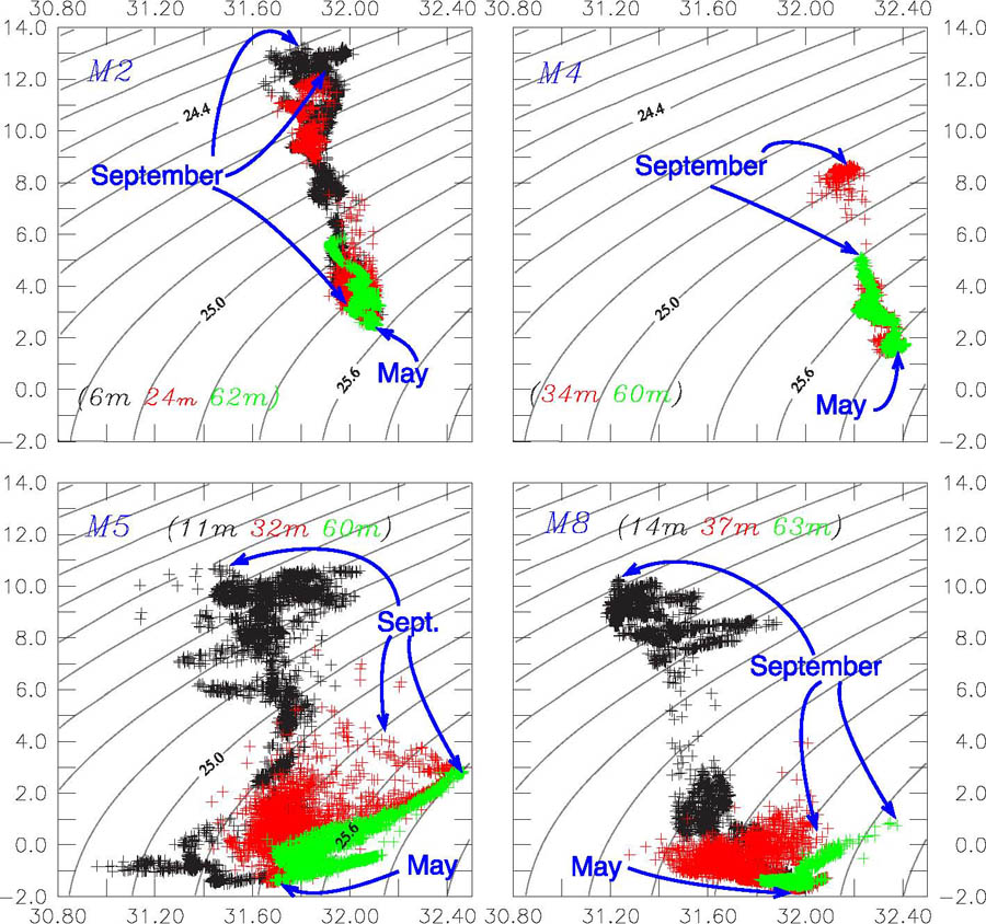
Fig. 12. Hourly temperature and salinity data from each moorings from three depths: near surface (black), mid-water (red), and near bottom (green). These panels show how the temperature and salinity changed over the course of the deployment (May to September). The near-surface instrument at M4 failed, so there are only two time series in that panel. The beginning of the time series (May) is indicated and the middle September is also indicated.
In May, at the beginning of the time series, the water at M5 and M8 was fresher than at M2 and M4, as a result of ice melt and the vertical mixing of this fresher water throughout the water column. Immediately after the water column became stratified, the temperature remained <−1°C at M5, but the surface freshened by ~0.6 psu, while the deeper water became more saline by ~0.4 psu. Ice persisted to the east and north of St. Matthew Island into June. As seen in the historical currents (Table 2), the flow at M5 is westward. Hence, the melting of ice behind St. Matthew would result in fresher surface water during late spring, which could then be advected past the mooring. By September the bottom salinity at M5 had increased to a concentration similar to that observed at M4 at the beginning of May.
At M8 there appeared to be periods of increased salinity in the surface waters. This occurred in mid to late summer, and the source is likely water that was advected northward along the 100-m isobath and then onto the middle shelf as seen in the trajectories of satellite-tracked drifters (Fig. 1). As the summer progressed the bottom instrument at M8 showed an increase of salinity accompanied by a slight warming. This increase in salinity at M8 was not as substantial as that observed at M5.
Cross shelf and along shelf advection were the cause of the temporal changes in salinity at the moorings. At M2 and M4 the changes were relatively small, since advection at these two moorings was weak during the summer (Stabeno et al., 2007). At M5 and M8, however, the near-bottom increase in salinity after June indicated the importance of advection at these locations. One distinct possible source of water is the Pribilof region, where bottom salinities (60–100 m water depth) range from 32.0 to 32.6 (Stabeno et al., 2007). Historically, drifter trajectories have revealed a weak on-shelf flow somewhere between M4 and M5 (Flint et al., 2002; Stabeno et al., 2006); this cross-shelf flow originates just north of the Pribilof Islands. Evidence for a cross-shelf flux was also found in changes in the spatial extent of the cold pool. A cold pool forms over that portion of the shelf, and as summer progresses this southern cold pool often becomes isolated from the northern cold pool, with warmer temperatures occurring somewhere between M4 and M5 (Wyllie-Echeverria, 1995a,b).
Historical reports of the broad-scale distribution of Bering Sea zooplankton communities also support the hypothesis that cross shelf advection of species occurs regularly on the shelf (e.g., Vinogradov, 1956; Motoda and Minoda, 1974). Zooplankton community distribution maps from the Russian literature describe an intrusion of oceanic organisms into the middle shelf domain north of the Pribilof Islands, inshore to about the latitude of Nunivak Island (Cooney, 1981; Coyle et al., 1996). The location of this intrusion is very similar to where we found the North–South Transition that was formed after the advection of slope or outer shelf water occupied the middle shelf. Similarly, Coyle and Pinchuk (2002b) detected oceanic and outer domain species near the inner front (ca. 50 m isobath) in this region. However, neither our spring nor late summer 2005 samples in that area showed significant concentrations of oceanic community species such as Neocalanus spp., Eucalanus bungii, or Metridia pacifica. The spring densities of these taxa (1–5 m−3) were greater farther south, between CTD Stations 94 and 118, perhaps due to on-shelf transport at Bering Canyon or transport across the shelf during spring before the frontal structure had become established.
These physical and biological observations support the hypothesis that the source of the warmer, more saline water observed at M5 and to a lesser extent at M8 was the outer shelf in the vicinity of the Pribilof Islands. The exact pathway is unknown. One possibility (supported by historical data) is that the weak onshelf flow north of St. Paul Island introduces water from the vicinity of the Pribilof Islands onto the shelf south of M5.
Go to Next section