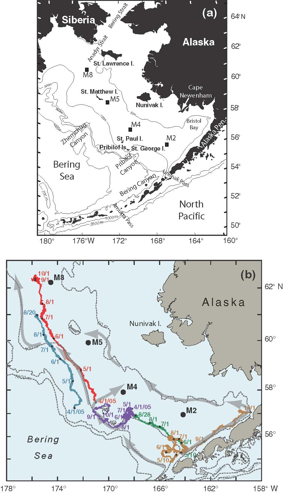
Fig. 1. (a) A map of the study region with bathymetric and geographic labels. (b) The locations of the four primary moorings (M2, M4, M5, and M8) are indicated. The arrows represent the mean flow over the shelf. Also shown are the trajectories from a series of drifters that were deployed in the region. The date of deployment for each drifter is given at the beginning of each trajectory and the position at the beginning of each month is indicated by month/day.

Fig. 2. Average percent ice cover in two bands of latitude, 62–63°N and 57–58°N, that stretch from the coast to the International Date Line and the shelf break, respectively. Averages were calculated from US National Ice Center data for each winter–spring (December, January–May), 1972 through 2005.
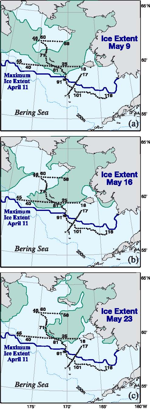
Fig. 3. Spring sea-ice extent during a three-week period in 2005. (a) Ice extent at the start of the cruise, (b) midway and (c) near the end of the cruise. The maximum ice extent was on April 11 and is shown as a thick black. The hydrographic stations for the spring cruise are indicated. The fall cruise occupied the same stations along the 70-m isobath. Moorings M4, M5, and M8 are at the intersection of the crossshelf lines and the 70-m isobath. M2 is at the southern terminus of the 70-m isobath.
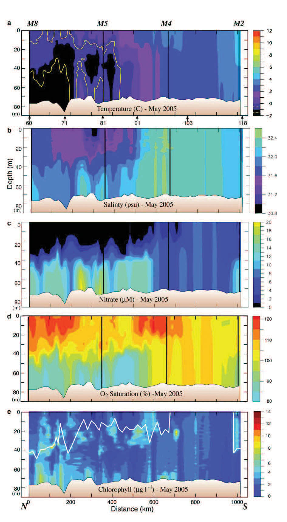
Fig. 4. Data collected along the 70-m isobath during the May 2005 cruise. The y-axes are depth. (a) Temperature, (b) salinity, (c) nitrate, (d) percent oxygen saturation and (e) chlorophyll. The vertical black lines indicate the position of the moorings. The distance between stations was ~20 km. The locations of specific stations are indicated at the bottom of the top panel. Nitrate was measured every ~10 m and at the bottom of each hydrographic cast. Since the stratification in the top panel was relatively weak, the 1°C isotherm is shown in yellow, and the −1°C isotherm is shown in white. The white line in the bottom panel is the mixed-layer depth (defined as the depth at which the temperature had decreased by 0.2°C).
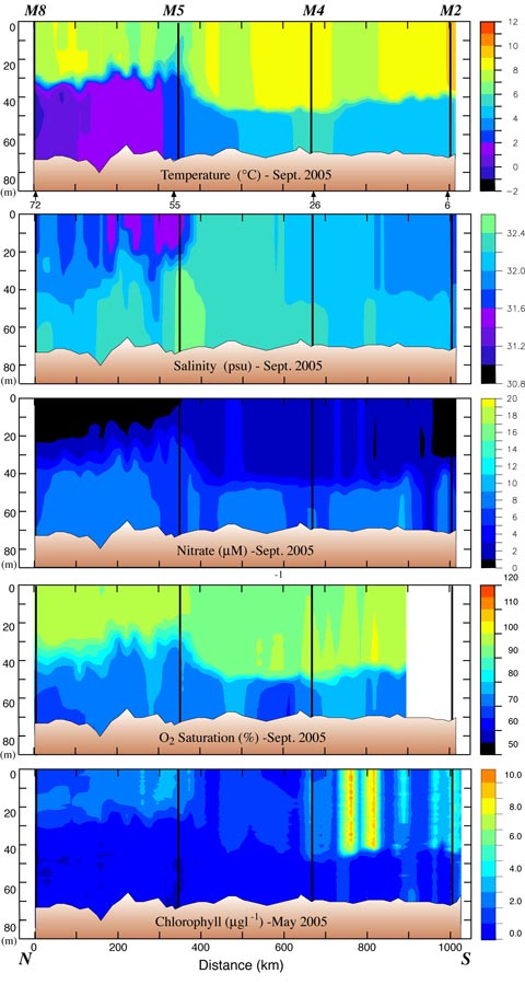
Fig. 5. Data collected along the 70-m isobath during the September 2005 cruise. The y-axes are depth. (a) Temperature, (b) salinity, (c) nitrate, (d) percent oxygen saturation and (e) chlorophyll. The black lines indicate the position of the moorings. The distance between stations was ~20 km. The locations of specific stations are indicated at the bottom of the top panel. Nitrate was measured every ~10 m and at the bottom of each cast.
Fig. 6. Panels a and c: Sigma-t along the 70-m isobath at 5 m and at 65 m. The rose shaded area indicates the portion of difference between the near-surface and near-bottom densities that resulted from just salinity and the gray-green shade indicates the portion that resulted from temperature. Panels b and d: Contours of the Brunt-Väisälä frequency along the 70-m isobath in May and in September.
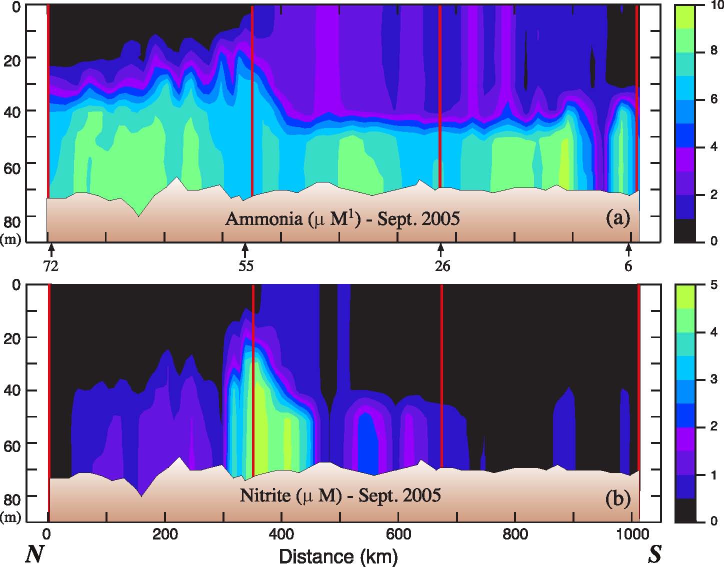
Fig. 7. (a) Ammonium and (b) nitrite in September 2005 along the 70-m isobath. The y-axes are depth. The vertical red lines indicate the position of the moorings.
Fig. 8. Percent total abundance of common zooplankton along the 70-m isobath. (a) spring, (b) late summer. A single sample was obtained at every other station along the isobath during spring, but in the late summer, replicate samples were obtained at the mooring site and at four stations forming a square around the mooring site (total of five stations). The exception is at M8 where a storm forced us to end operations early. A single sample was collected at that mooring site.
Fig. 9. Hydrographic section along the St. Matthew Island transect during the May 2005 cruise: (a) temperature, (b) salinity, (c) nitrate, (d) percent oxygen saturation and (e) chlorophyll. The y-axes are depth. The domains are indicated at the top of the plot and the locations of specific stations are indicated at the bottom of each panel. Nitrate was measured every ~10 m and at the bottom of each cast.
Fig. 10. Time series of wind speed and water temperature during 2005. (a) NCEP wind speed at M2 (black) and M8 (red), (b) through (e) contours of water temperatures at M8, M5, M4, and M2, respectively. The yellow lines at M2 and M8 are the estimates of chlorophyll concentration (μg l−1) derived from the fluorometers. The time period shown is May 1 through September 30, 2005.
Fig. 11. Time series of atmospheric and oceanographic data from M2 during the month of May. (a) PAR measured at 3 m on the tower of buoy and (air temperature) − (surface water temperature). (b) The friction velocity (u*3) from the hourly winds measured at the buoy. Wind stress was calculated using Large and Pond (1981). (c) chlorophyll at 11 m and the nitrate at 13 m. (d) Temperature was measured at every ~3–4 m and the hourly data were contoured to show temperature structure. (e) Shear measured by a nearby ADCP.
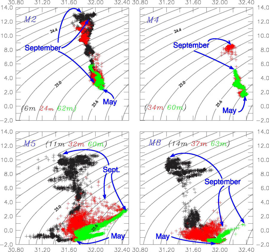
Fig. 12. Hourly temperature and salinity data from each moorings from three depths: near surface (black), mid-water (red), and near bottom (green). These panels show how the temperature and salinity changed over the course of the deployment (May to September). The near-surface instrument at M4 failed, so there are only two time series in that panel. The beginning of the time series (May) is indicated and the middle September is also indicated.
Go to Abstract