Climatology of Solomon Sea Currents, Temperature and Salinity
Data
Latest update (May 2020)
Northern track (eastbound)
- Mean (108 KB)
- 12-month annual cycle (1.2 MB)
Southern track (westbound)
- Mean (108 KB)
- 12-month annual cycle (1.2 MB)
Download all 4 files as zipped NetCDF [SolomonSea_Climatology.zip] (2.3 MB)
Included variables are: in-situ temperature, practical salinity, potential temperature, potential density, binned transport (as function of depth and cross-basin distance), vertically-averaged velocity (directly measured), and pseudo-velocity (an estimate of the magnitude of equatorward flow derived from the cross-track absolute geostrophic velocity, see description in Methodology). The NetCDF files are CF-1.7 and ACDD compliant.
How to cite
- Full data set of glider measurements including temperature and salinity profiles, and vertically-averaged absolute velocity:
Davis, R. (2016). Solomon Sea Ocean Transport from Gliders [Data set]. Scripps Institution of Oceanography, Instrument Development Group. doi: 10.21238/S8SPRAY2718 - Climatology of geostrophic currents, temperature and salinity shown on this webpage:
Kessler, W.S. and H.G. Hristova (2021). Climatology of Solomon Sea currents, temperature and salinity measured by glider [Data set]. Scripps Institution of Oceanography, Instrument Development Group. doi: 10.21238/S8SPRAY2718B
Reference
Kessler, W.S., H.G. Hristova and R.E. Davis, 2019: Equatorward western boundary transport from the South Pacific: Glider observations, dynamics and consequences. Progress in Oceanography, 175, 208-225, doi: 10.1016/j.pocean.2019.04.005
Corresponding author's email (ask for copy of paper): william.s.kessler@noaa.gov
Methodology
Only the segments of glider missions making complete transects between Papua New Guinea (PNG) and the Solomon Islands (SOL) are considered here. The glider samples the Solomon Sea in a clockwise loop, naturally forming two separate tracks: a northern track (with eastbound sampling) and a southern track (with westbound sampling). The two tracks have distinct velocity characteristics. The annual cycle is thus computed separately for each track. All data were low-pass filtered to remove small scales not relevant for geostrophy prior to computing a 12-month average annual cycle and its mean (see Kessler et al. 2019, section 2.2 for details).
To construct consistent and comparable transects from the irregular glider tracks, data are reported as a function of the cross-basin fraction ϕ, varying between 0 at PNG and 1 at SOL, where contours of constant ϕ align with the general direction of the mean flow in the Solomon Sea (see gray contours of ϕ in Figs. 1 and 2 below, and Kessler et al. 2019, section 2.3 for details). All cross-section data are binned vertically in depth (Δz =10m) and horizontally in ϕ (Δϕ = 0.05). A discontinuity occurs at depth 700m since missions sampling to 1000m began in mid-2013 (see Kessler et al. 2019, section 2.1 for details).
Pseudo-velocity
Absolute depth-averaged vector velocity is inferred by the glider as an average over each dive, covering about 5km horizontally and 1000m vertically, and taking about 5 hours. The inferred absolute current velocity is the difference between the actual displacement (between the observed dive and resurface positions) and the displacement predicted by a flight model that estimates the glider’s motion relative to the water (Sherman et al. 2001; Davis et al. 2012). Temperature and salinity measured during the dive give geostrophic shear (perpendicular to the glider track) relative to the dive depth. These can be combined to produce the absolute cross-track geostrophic velocity as a function of depth and along-track distance.
Computations (such as finding the average or annual cycle at a chosen ϕ) using this cross-track velocity could be misleading, since the track orientation is highly variable and does not repeat from cross-section to cross-section. Instead we introduce the pseudo-velocity, an estimate of the magnitude of along-ϕ equatorward flow in the Solomon Sea. It is defined as the along-ϕ velocity whose component in the cross-track direction at each profile location equals the cross-track velocity (see Kessler et al. 2019, section 2.3). Although not a measured quantity, the pseudo-velocity allows averaging over the irregular tracks, using ϕ as a cross-basin coordinate. It can be estimated for all profiles using only the cross-track velocity and the track orientation with respect to ϕ-contours. The pseudo-velocity has units of velocity and by definition leads to the same coast-to-coast transport as the cross-track velocity. Overall, the pseudo-velocity is a suitable estimate (not a direct measurement) of the along-ϕ equatorward flow in the Solomon Sea (see Kessler et al. 2019, section 2.3 for details).
The spatial structure and annual cycle of the pseudo-velocity are similar to those of the binned transport. Both are included in the distributed files since both may be of interest. The bin-averaged pseudo-velocity shows the magnitude of equatorward flow in units of velocity, while the sum of the binned transport for a cross-section gives the total transport for that cross-section (in Sv).
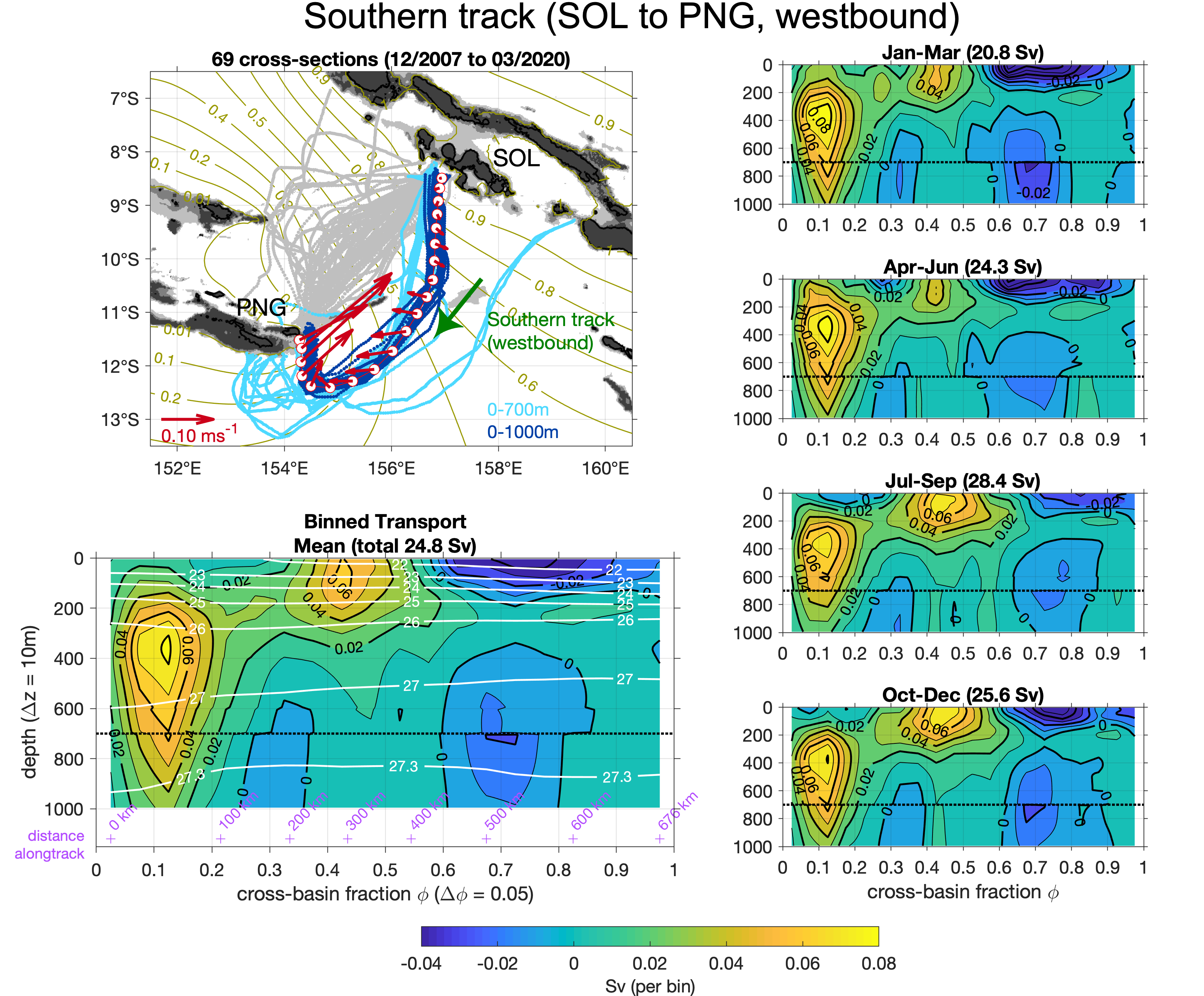
On the southern track, the velocity structure shows two distinct cores: shallow mid-basin inflow, and a much thicker western boundary current, the New Guinea Coastal Undercurrent (NGCU), that extends with great magnitude to and below the sampling depths of 700m and 1000m. Positive values indicate equatorward transport. Transport is maximum in Jul-Sep, and weakest in Jan-Mar, varying by ±3 Sv from its mean of 25 Sv. The annual cycle of transport is largely controlled by the variations of the mid-basin inflow strength.
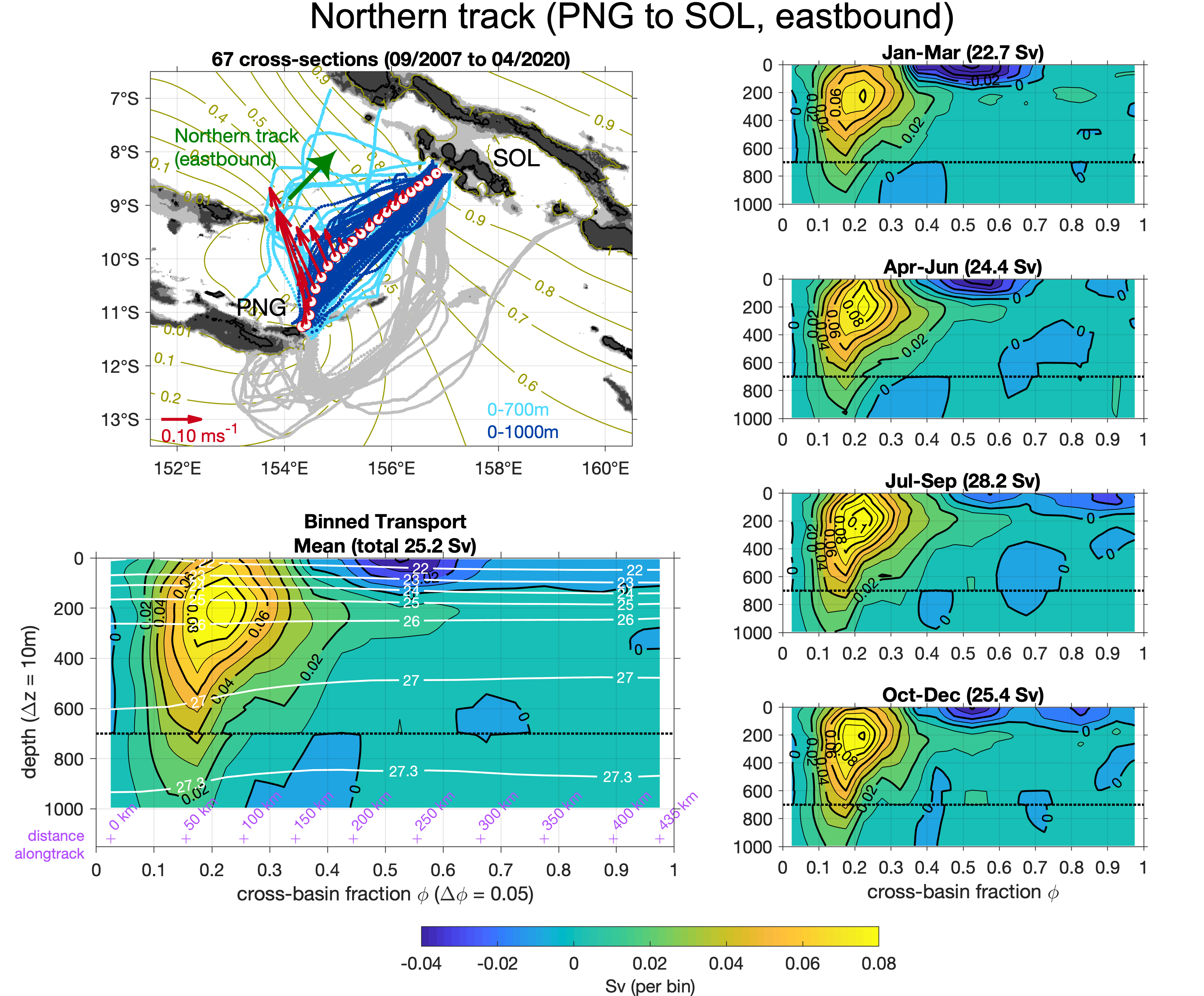
On the northern track, the velocity structure shows a single, broader maximum in the west where the NGCU and the mid-basin inflow have apparently merged into a single current on the PNG side. Positive values indicate equatorward transport. Transport is maximum in Jul-Sep, and weakest in Jan-Mar, varying by ±3 Sv from its mean of 25 Sv.
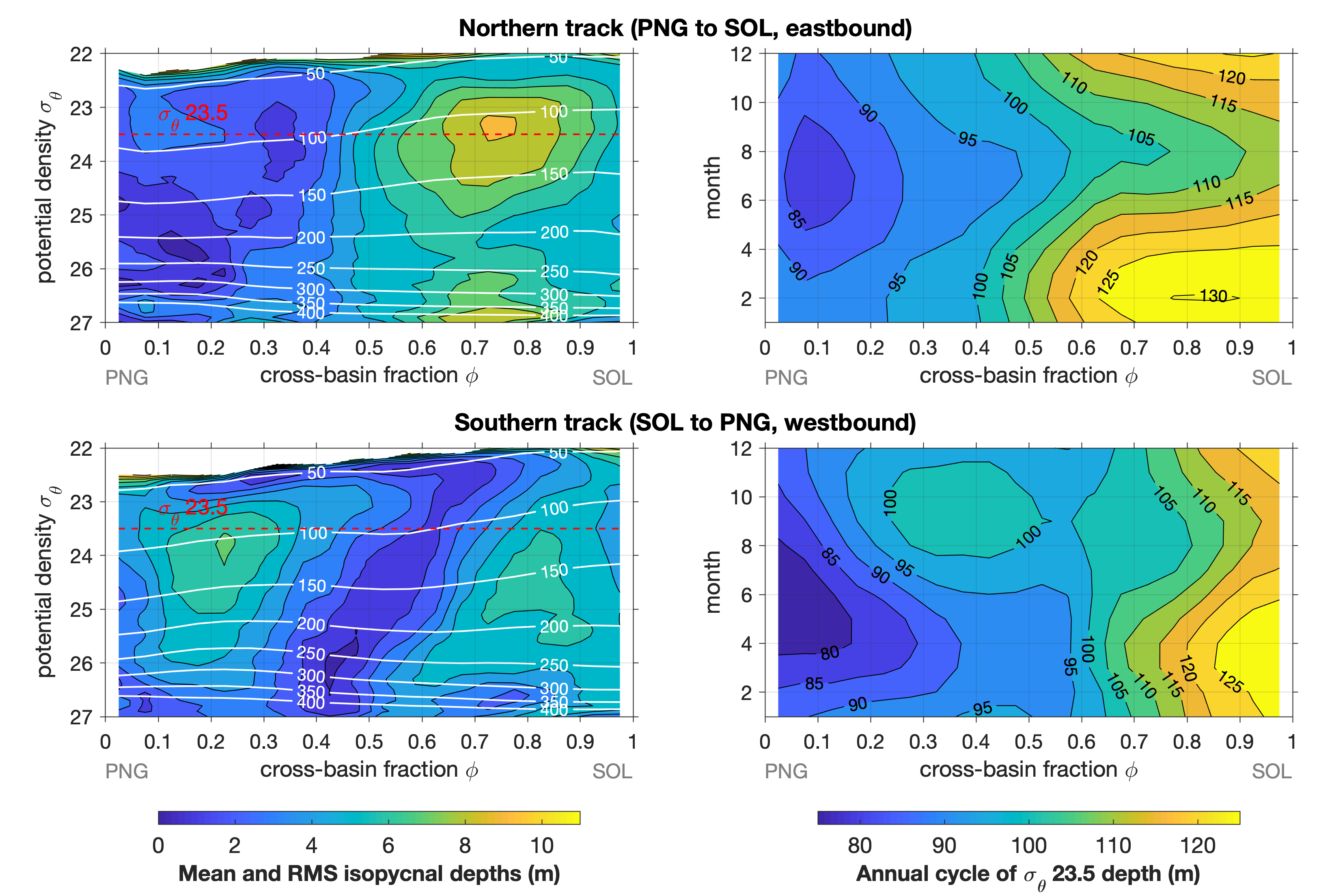
Isopycnal depth fluctuations are much larger on the Solomon Island side, largely controlling the pycnocline slope across the basin. Possible mechanisms for this variability and the role of local versus remote forcing are discussed in Kessler et al. 2019 (Section 5.3).