U.S. Dept. of Commerce / NOAA / OAR / PMEL / Publications
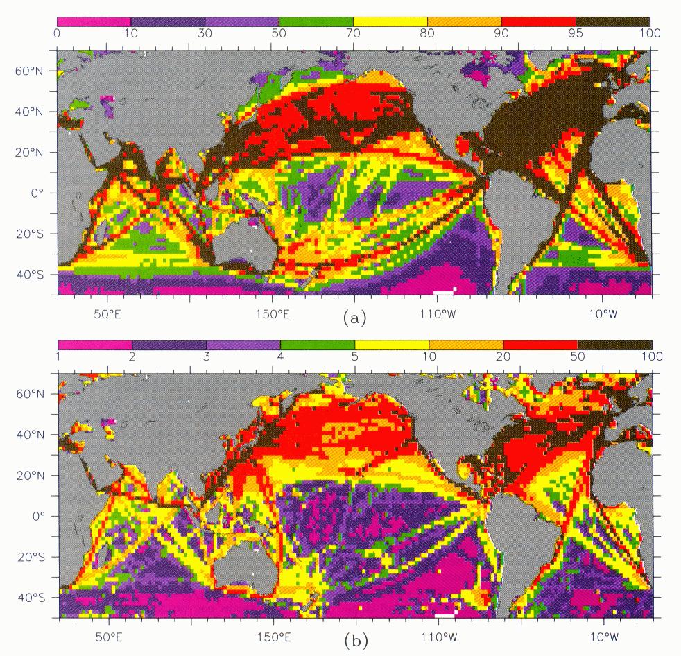
Due to the considerable event to event variations, it is not feasible to describe in detail the features of each ENSO event in this data set. Instead, in this section, we show the relationship between aspects of the Schematic Composite and the individual ENSO events. The simplest way to examine the generality of features in the composite is to examine time series of SLPA from regions near the extrema in the composite. We evaluate simple area averages over rectangular regions (10░ ū 8░ in most cases) as close to the extrema as possible. This spatial averaging is comparable to the RC spatial filtering used in the composite. It is not always possible to construct useful time series centered on the extrema, due to data limitations. We experimented with time-filtering the area averages in a variety of ways; the main results are not sensitive to the choice of smoother, provided its half power point lies between three and six months period. Results are presented here using a 5 month triangle smoother. This smoother has a half-power period of 7.6 months and better side-lobe characteristics than the common three running mean (e.g., Chelton and Davis, 1982), which has a half power period of 6.4 months. Figure 8 shows some of the regions over which we evaluated these time series; the coloration indicates the percentage of months having data within the region (as in Fig. 1). In addition, we examined every 10░ x 8░ region with enough data north of 20░N in the Pacific. Note the paucity of data in the central south Pacific and the western equatorial Pacific regions.
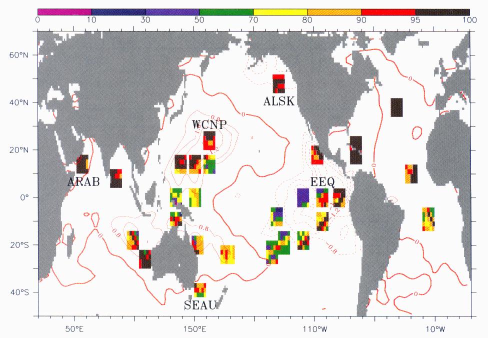
Fig. 8. Location of some of the time series regions used to assess the robustness of the composite, superimposed on December(0) SLPAN. Regions whose time series plots are presented in Section 5 are labeled. Coloration indicates the percentage of months with data as in Fig. 1a.
We present time series normalized by their own standard deviation. This is very similar to the composite normalization, and we use the same notation, with the understanding that, for this section, SLPAN = SLPAREGION AVERAGE /TS. Because the time series regions have slightly different smoothing than the smoothing used in the composite construction, SLPAN values presented here are not identical with composite values at the central location of each region. Results for each region are presented as in Fig. 9. The first two panels present the time series of SLPAN between 1946 and 1994, with ENSO Year(0)s indicated by bottom brackets. This panel helps the reader see if the behavior found during the composite exists during each El Ni±o period and whether it occurs in other periods. The standard deviation (TS) is written in the upper left hand corner of the first panel, so it may be used to convert SLPAN to SLPA if desired. The third panel presents an overlay of SLPAN for each ENSO period, from Year(-1) to Year(+1). In the following discussion, we use the boreal seasonal notion defined in section 4.3. Recall that the only aspects of the composite that exhibit both local and field significance in excess of the 95% level are the EEQ low and the WCNP high; we consider time series in these regions first.
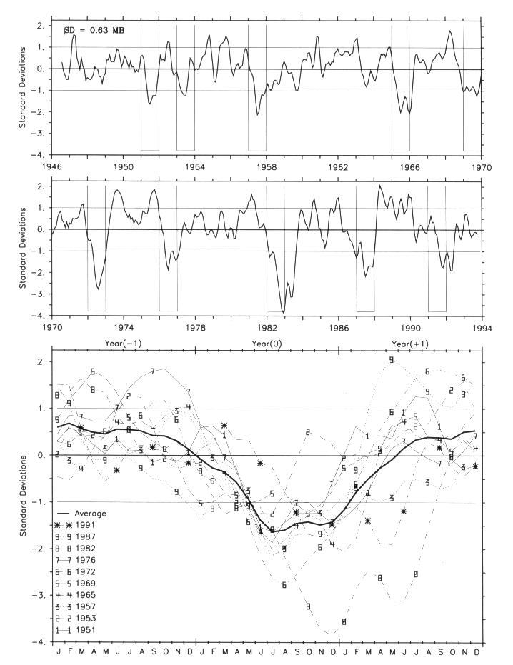
Fig. 9. The EEQ SLPAN time series averaged over 108░W to 98░W, 4░S to 4░N and time smoothed by a 5-mo triangle filter (see section 5). The top two panels present the time series, 1946-1993. Bottom brackets identify each ENSO Year(0) . The bottom panel presents an overlay of SLPAN for each ENSO period from Year(-1) to Year(+1). The different ENSO events are indicated by number: 1 = 1951, 2 = 1953, 3 = 1957, 4 = 1965, 5 = 1969, 6 = 1972, 7 = 1976, 8 = 1982, 9 = 1987, * = 1991.
Our time series analysis reveals that the most robust pattern found in the composite is the eastern equatorial Pacific low (EEQ) during Sp(0) through W(0) (Fig. 9). We examine the behavior of this feature by averaging from 108░W to 98░W, 4░S to 4░N. Every ENSO period shows one or more negative SLPAN peaks exceeding -1. The major ENSO events, 1957, 1965, 1972, and 1982 each have EEQ < -2 for at least two months. The largest signal was in 1982, when EEQ < -3 was observed. The events of 1965, 1982 and 1991 also had EEQ < -1 during Sp(+1). The 1982 event was the only one in which EEQ < -1 continued past Sp(+1). In non-ENSO periods, EEQ is never < -1 for three consecutive months. Thus EEQ < -1 constitutes a necessary and sufficient criteria for picking out the ENSO periods in this record. The area average can be moved several degrees in any direction without severely altering these results.
While EEQ exhibits a negative peak < -1 during each ENSO period, the characteristics of EEQ vary from event to event. Consider the overlaid ENSO SLPAN (bottom panel of Fig. 9). Typically, EEQ first reaches -1 during the period June-July(0), with 1969 and 1987 occurring significantly earlier and 1991 later. EEQ's behavior during the major ENSO periods can be grouped into two main types. In the first there is a single negative extremum (1953, 1955, 1957, 1972); in the second there are two negative extrema (1951, 1965, 1976, 1982, 1987 and 1991). 1969 is unique in having a broad flat negative extremum, lasting nearly a year.
The next most rigorous connection between a composite feature and individual events is the WCNP high from F(0) into Sp(+1). Figure 10 presents time series for WCNP based on an area average over 158░ to 168░E, 20░ to 28░N. We see that composite type behavior, with peak values of WCNP > 1, is found in the events of 1951, 1957, 1965, 1972, 1982, 1987, and 1991. Departures from composite behavior are found in the 1953 and 1969 events, which have no positive peak during F(0) - Sp(+1), and in the 1976 event which has weakly negative values during this period. The weakest WCNP maxima occur in the 1951 and 1953 events, with WCNP about 1.5. Most events have maximum WCNP values around 2 and the 1982 event has a maximum WCNP of almost 4. Two non-ENSO periods, 1959 and 1973, have positive extrema above 1.5. Overall, WCNP > 1.5 values are typical of ENSO periods and infrequent during non ENSO periods.
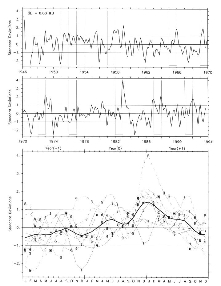
Fig. 10. Same as Fig. 9, except for the WCNP region, 158░ to 168░E, 20░ to 28N░.
The remaining aspects of the composite--the southeastern Pacific (SEP) low, the northern Australian (NAUS) high, the southeastern Australian (SEAU) low, the Arabian Sea (ARAB) high, and the Alaskan coast (ALSK) low--are of only marginal significance. While they exceed our local significance criteria at the 99% level, they do not meet our stringent field significance test at this level. As might be expected, individual events show more variability for these aspects than they do for EEQ or WCNP. We shall only discuss the SEP and NAUS signals, for reasons mentioned below, but we present SLPAN timeseries averaged over regions representative of the other features: for SEAU (Fig. 11) 150░ to 160░E by 42░ to 36░S; for ARAB (Fig. 12) 52░ to 62░E by 10░ to 18░N; for ALSK (Fig. 13) 144░ to 134░W by 44░ to 52░N.
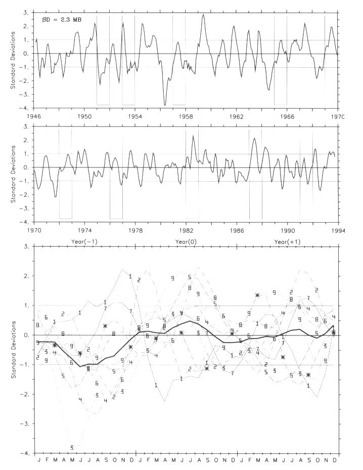
Fig. 11. Same as Fig. 9, except for the SEAU region, 150░ to 160░E, 42░ to 36░S.
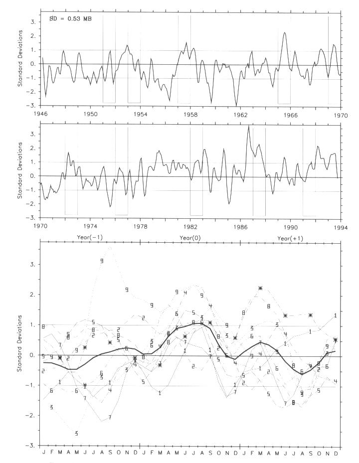
Fig. 12. Same as Fig. 9, except for the ARAB region, 52░ to 62░E, 10░ to 18░N.
The SEP low center forms with EEQ in Su(0) but lasts for only two seasons. The SEP composite values greatly exceed the 99% significance level locally, having comparable extrema to EEQ, but SEP is not large enough in area to obtain field significance. We examined the behavior of time series in three different regions near the SEP composite extremum but were limited to areas with the best data coverage. We find the different time series differ non-trivially, suggesting that the data are at best marginal to study this aspect of the composite in detail. Larkin and Harrison (1996) presents the various time series. The only clear results from these series are that the composite SEP signal results substantially from very large values during the 1982 and 1991 El Ni±o events, and that values in excess of -1.5 occur in about half the El Ni±o events sometime during Yearr(0) in this general area. Data density is a serious issue for this signal; it is possible that with improved data a more robust result might be found. However, the above results are the strongest permitted by these data.
The NAUS high found in Su, F, W(0), is spatially diffuse in the composite, extending from the Australian coast into the Maritime continent, with extrema occurring in many distinct locations at different times. As a result, it is not surprising that the time series averages reveal that the NAUS high has considerable small scale structure. Location of the areal average severely affects the time series pattern found; for this reason no figure is shown, instead the reader is referred to Larkin and Harrison (1996). The NAUS high results primarily from large signals during the 1972, 1982, and 1991 events; 1987 also exceeds the positive significance threshold, but has weakly declining values throughout these seasons. The remaining events show different characteristics depending upon the region chosen, but frequently have weakly opposite behavior to that found in the composite. Several non-ENSO years show positive values near our significance threshold. The signal in regions off western Australian is typically more robust.
The remaining features of the composite are less spatially diffuse and have better data coverage than SEP and NAUS. Figure 11 reveals that the SEAU negative feature during Sp, Su(-1) results primarily from strong negative extrema during the 1957, 1965, and 1972 ENSOs; 1953 and 1969 also exceed -1 during the time of the negative composite feature. The dominant event is 1957, when the minimum approached -3.75. The 1951 event shows behavior strongly opposite to the composite, while the events of 1976, 1982, 1987 and 1991 either never reach the negative significance level or go weakly positive over the months of interest. Negative values of -1 or less are not uncommon during non-ENSO periods, occurring more than a dozen times. The strongest statement that can be made about SEAU is that it is not uncommon for ENSO events to show this low off Australia in year(-1).
Figure 12 shows the time series (ARAB) of the Arabian Sea high during Sp(0) and Su(0). A maximum exists in this time series during each El Ni±o period except for the event of 1953, but in several of the events the peak is less than or barely unity. The major contributors to the composite peak are the 1965 and 1987 events, with maxima of about 2. Positive values larger than unity exist during non-El Ni±o periods of 1968, 78, 79, 83, 84, 86 and 89; the past twenty years exhibit this behavior far more frequently than the first twenty years of our record. Overall we may summarize the robustness of this feature by stating that it is found, to some degree, in almost every El Ni±o period, but that it also occurs with some frequency during non-El Ni±o periods.
Figure 13 indicates that the ALSK negative composite feature during season W(0) results primarily from very negative values during the 1957, 1982 and 1991 events. 1953 and 1969 also contribute somewhat to the composite feature, although their extrema occurred more during Su, F(0) than during W(0). 1951, 1972, 1976, 1987 had weakly positive values while the composite was negative. Many non El Ni±o periods exhibit ALSK < -1.5. This feature is occasionally strongly present during ENSO, but is not truly typical.
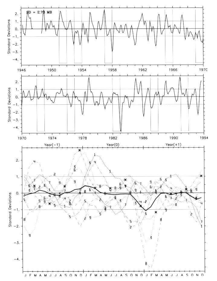
Fig. 13. Same as Fig. 9, except for the ALSK region, 144░ to 134░W, 44░ to 52░N.
It is of interest to examine the time series of the Troup SOI in the format of the composite feature time series (Figure 14). The composite behavior of the Troup SOI is shown in the heavy black line in the third panel; in the spirit of our previous composite discussion we say that low values of SOI between Su(0) and (arguably) Sp(+1) are the composite event feature associated with SOI. The upper panels show that this behavior is not uniquely associated with ENSO periods; the ENSO event periods of 1951 and 1969 do not reach the marginal significance level for composite SOI behavior, two other ENSO periods show very marginal SOI signal (1957, 1976), and the non-ENSO periods of 1946, 1977-78 and 1990 have substantially negative values for at least one season. 1963 and 1993 also show composite type SOI behavior; following the RC convention (as well as that of Deser and Wallace, 1987) 1963 is not an ENSO period, but the status of 1993 has yet to be settled in the literature. In the language we have used for the other composite signals the SOI behavior is relatively robust; all events have SOI < 0 during the period identified by the composite and many have SOI < -1 during this period the composite, but this behavior is not uniquely associated with ENSO periods. The SOI feature is clearly less uniquely associated with ENSO periods than EEQ.
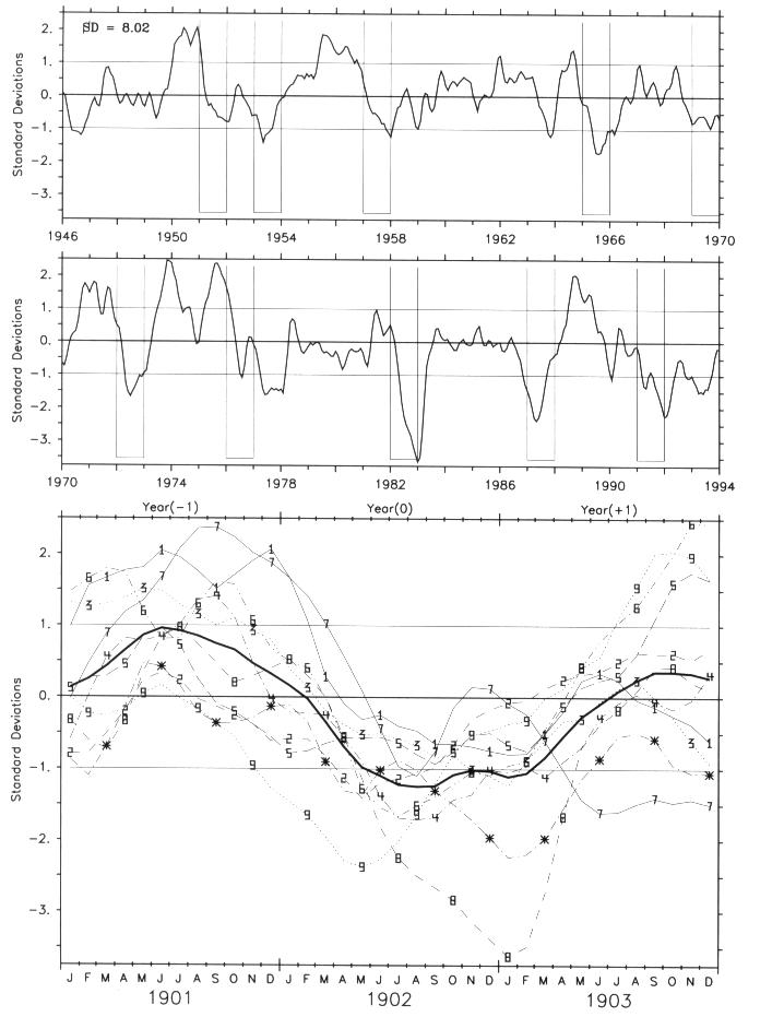
Fig. 14. Same as Fig. 9, except for the Troup SOI, smoothed and normalized as in Figs. 9-13. See section 5.
Return to previous section or go to next section