U.S. Dept. of Commerce / NOAA / OAR / PMEL / Publications
We have constructed composite maps for the 60-month period spanning January of Year(-2) to December of Year(+2), where Year(0), as in RC, is the year of South American coastal "El Nińo" warming. Years(0) are taken to be 1951, 1953, 1957, 1965, 1969, 1972, 1976, 1982, 1987, and 1991. The choices of 1951-1972 match those of RC. We chose 1987 over 1986, as the patterns are more consistent with other ENSO events if we identify 1987 as Year(0) for this event rather than 1986. Using 1986 instead has no significant effect on our composite. The Year(0) choices of 1976, 1982 and 1991 for the other post-1972 ENSOs should not be controversial.
We began our efforts to construct a composite by exploring the effect of normalizing each ENSO event by some maximum amplitude or amplitude difference before averaging events together to form the composite. RC did not perform this normalization, and it has been known for some time that their composite is strongly influenced by the 1972 event, both because of its large amplitude and because more data were available from this event than from the others in their data set. We have been unable to devise a defensible event normalization factor, however, because there are large data gaps spanning the regions of the largest ENSO signals.
A second possible preparation for compositing involves allowing the "zero time" to vary from event to event, since different events seem to have somewhat different phasing relative to the seasonal march. We found no satisfactory strategy for introducing a phase shift; the same data limitations that make it too difficult to define a useful amplitude factor make it even harder to deal with issues of phase. We composite by averaging together the same calendar month of each event, as was done by RC.
The next challenge was to illustrate the features of the global ENSO signal. These features are not easily discerned because the mean SLP field has substantial spatial structure and a significant seasonal march in many areas (see appendix). Examination of ENSO from SLPA fields also presents significant interpretation challenges, since the extra-tropical interannual variability is typically significantly greater than the tropical variability (see section 2). For example, 2 mb in SLPA is a very large tropical signal, but is negligible in middle latitudes. After some exploration, we decided to present the composite in terms of a variance-normalized SLPA. We normalize the RC-smoothed SLPA fields by the standard deviation of the RC-smoothed SLPA time series at each point (see section 2 and Fig. 3c). Contours shown here are in units of regional non-seasonal standard deviation of SLP. We shall denote anomalies normalized in this way as SLPAN, reserving SLPA for unnormalized anomalies (in mb).
This normalization is not traditional for large scale descriptive work, but is similar, although not identical, to normalizations used by van Loon and Shea (1985) and van Loon and Labitzke (1987). We use it here because: 1) it emphasizes the relative importance of the ENSO signal compared to the total non-seasonal variance, 2) this field has little small scale spatial structure of its own (see Fig. 3c), and 3) it facilitates consideration of statistical significance (see below). SLPA composite maps are presented in Larkin and Harrison (1996).
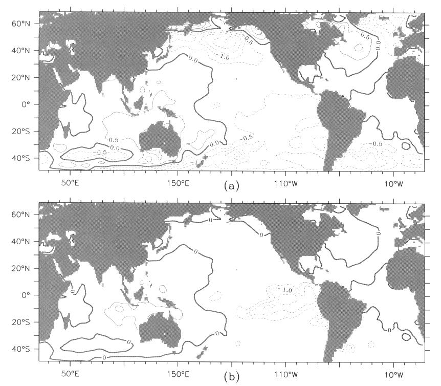
The effect of examining SLPAN instead of SLPA is clearly shown in Fig. 5. The extra-tropical signal is greatly reduced, allowing the tropical signal to stand out. A further benefit of this normalization is that much of what we believe to be statistically insignificant variability poleward of 40°S is filtered out in SLPAN. An unappealing aspect of SLPAN is that it cannot be related simply to wind anomalies. A subsequent paper, Harrison and Larkin (1996), will present wind and SST results and their relation to SLP.
Fig. 5. The effect of normalizing SLPA by Fig. 3c to create SLPAN. Composite September(0) as an example. a) SLPA, contoured every 0.5 mb. b) SLPAN, contoured with zero (heavy line) and then ±0.8, ±1.0, ±1.2, ±1.4, ±1.6, etc... The ±0.8 contours correspond to a local Normal-z 99% significance level. Significance levels of contours are discussed in Section 4.1.
The matter of statistical significance also merits discussion. We check for local (spatial point) significance of the composite using several methods, including the Normal-z statistic, and the Student's t-test (which differ in the standard deviation used). We find comparable results using each method. We shall present the local significance level in terms of the Normal-z statistic as our normalized sea level pressure, SLPAN, and the Normal-z statistic are related by:
where n is the number of events in the composite (10), and SLPATS is the standard deviation of the RC-smoothed SLPA time series at that point.
However, we note that determination of significance levels in this way is complicated by the lack of data in certain regions and the fact that both the Student's-t and Normal-z statistics assume underlying normal distribution. To address the effect of possible non-normal distributions, we have employed a Bootstrap technique which uses only the data distribution itself (Efron and Tibshirani, 1991) to determine various confidence levels. We apply our Bootstrap method to each spatial point separately, choosing with replacement a time series from the original and then calculating a Bootstrap SLPAN. We used B = 10000 iterations to determine our Bootstrap confidence levels. For confidence intervals up to 99% we find good agreement between the Bootstrap calculations and the Normal-z statistic. This is fortuitous for two reasons: 1) confidence intervals based on z are universal spatially, whereas the Bootstrap intervals are not; 2) the Normal-z statistic is easily related to our normalized sea-level pressure anomaly, SLPAN, as shown above. Hereafter, all mention of local significance levels are to be understood as relating to the Normal-z statistic.
The Normal-z 99% confidence level (the first non-zero contour shown on the composite maps) is SLPAN > z99/(n)0.5 = 0.81. We do not show the 95% confidence level here as little below the 99% level (and much above the 99% level) is found to have field significance. Instead, we refer to the accompanying technical memorandum (Larkin and Harrison, 1996) for presentation of lower local confidence intervals. Note that this is only a test of point significance; for an idealized random distribution we expect 1% of the map to be at or above this level (both positive and negative) on any given composite month. Other levels of SLPAN shown on the composite maps are 1.0 , 1.2, 1.4, and 1.6. While these levels are necessarily above the 99% local confidence level, the exact local significance varies with location on the globe and can only be approximated through the Bootstrap test above. We do not believe that all of the patterns associated with the 99% confidence level are significant in a field (global) sense but find that signals at the 1.0 level and above tend to have enough large scale coherence and temporal stability to be plausible.
Statistically, there are many ways to check for field significance of a given structure in the composite. The simplest is to calculate the percentage of the field in a given month that is locally significant (as above) and then determine the probability that this percentage would be observed randomly (Livezey and Chen, 1983). To do this, some assumption must be made about the spatial interdependence of the field to determine the number of independent spatial points. We have calculated the field significance using a range of assumptions, from an optimistic 21° × 18° (the half power point size of our spatial smoother), to a rather cautious 42° × 36° for each independent point. The local significance criteria checked for field significance can also be varied--a very large scale low level signal (low local confidence level) may still have a high field significance level. We have checked a variety of local significance criteria, from the 50% (zero contour) to the 99.5% levels. Only two components of the composite have field significance at the 95% confidence level in these calculations: the western central north Pacific high (labeled WCNP), and the eastern equatorial Pacific low (EEQ) as will be discussed in the next Section. We note that while we use present results at the 99% local confidence level, we use a 95% confidence level as our field significance criterion. This is due to the fact that our field significance calculation is a stringent test in that it does not take into account the spatial structure, temporal coherence, or other noteworthy characteristics of the signal. More aspects of the composite may be found to be significant using other, tailored tests.
We call signals with field significance at or above 95% "significant" signals. These signals will be shown to be reasonably robust (all or most ENSOs exhibit this behavior). "Marginally significant" signals, ones that have local significance and some spatial and temporal coherence but that do not meet the stringent field significance test above, seem to arise when one or more ENSOs have the sort of behavior found in the composite, or when there is considerable variation in the timing of a particular feature among events. Marginally significant signals occur much more frequently in the composite. We discuss the robustness of our composite results when we examine the event to event behavior in Section 5.
We present selected results of our composite SLPAN analysis in Figs. 6a-o. These selected fields include data from April(-1) through August(-1) and April(0) through May(+1). Please see Larkin and Harrison (1996) for the full July(-2) through June(+2) composite maps. Each smoothed map shown here includes data from a 3-month running mean (section 2), but is referred to by its center month. We show the zero contour and contours of amplitude ±0.8 (99% confidence level), ±1.0, ±1.2, ±1.4, ±1.6. Signals within the 99% interval (-0.8 and 0.8) are not contoured because we judge them unlikely to be significant (see above). Labels are given to features that both meet the 99% local significance level and show some robustness when time series are scrutinized; these features are also discussed in section 5.
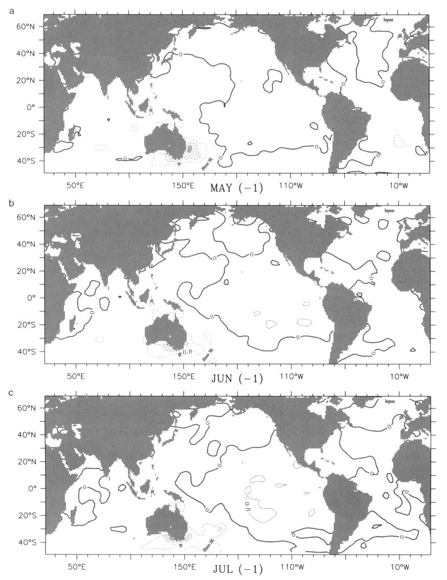
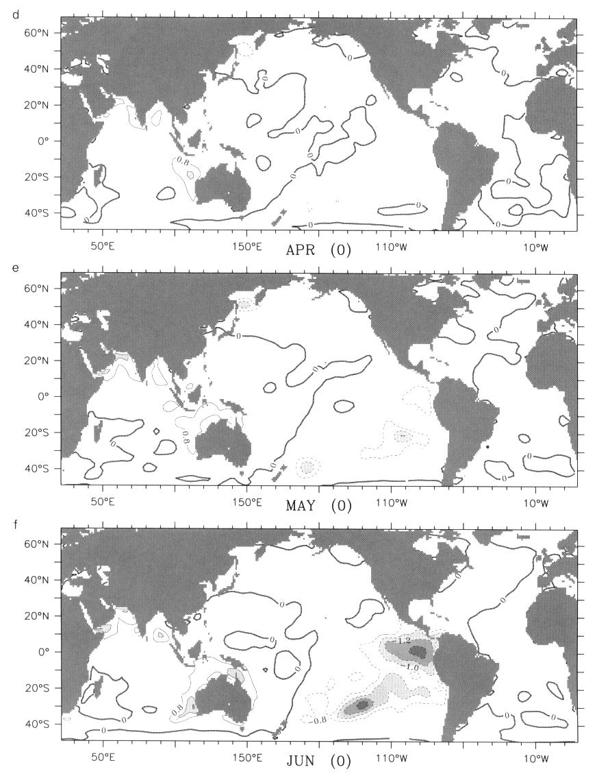
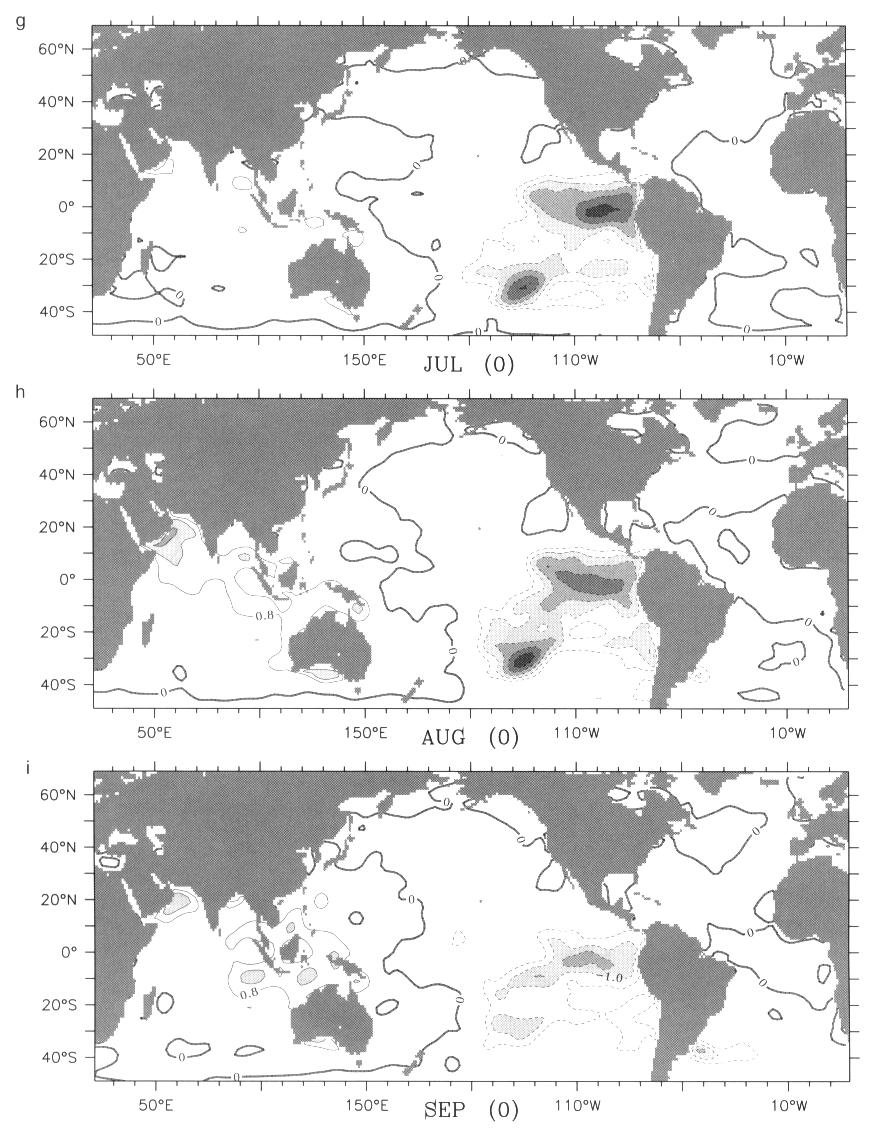
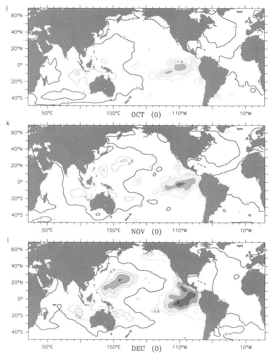
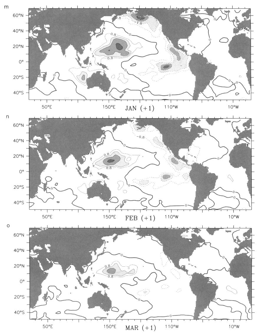
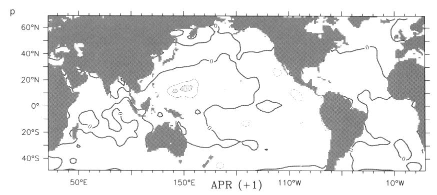
Fig. 6. The evolution of the SLPAN El Nińo composite, May(-1) through July(-1) and April(0) through April(+1). No significant signals are seen between August(-1) and March(0). Contours are as in Fig. 5(b). SLPAN in excess of ±1 is shaded. See Section 4.2 for discussion of composite features.
The first marginally significant feature (SEAU) is an area of low SLPAN off the southeast coast of Australia in early Year(-1). SEAU appears, nearly fully developed, in May(-1), and intensifies somewhat through July(-1) (Figs. 6a-c). The extreme SLPAN value is nearly -1.2 and occurs over the Tasman Sea in July(-1). While SEAU reaches its extreme value, the greater eastern tropical Pacific SLPAN becomes slightly positive. In a few small regions between 160°W and 130°W, 30°S to 10°S values near +0.8 occur but do not persist. From August(-1) to September(-1) SEAU weakens. While this region continues to have small negative SLPAN, it no longer meets local significance criteria.
Between August(-1) and March(0) there are no other signals of even marginal significance, and these periods are not shown here. During this time, the Pacific north of 30°N remains positive while south of 30°N the Pacific becomes negative. Evidently the composite analysis can contribute little to an understanding of the surface SLPA signals over these months, which are of crucial interest for ENSO forecasting.
In April(0) (Fig. 6d) another marginally significant signal begins: scattered areas from Australia to the Arabian Sea develop positive SLPAN values greater than 0.8. Through June(0), the area northwest of Australia expands around the edges of the continent, and the Arabian Sea signal (ARAB) expands slightly. These signals diminish in July(0) before reaching their maxima in extent and amplitude in August(0). At this point, they connect to form a SLPAN ridge that extends from the Arabian peninsula to Australia, with maximum values greater than 1.0 in many areas and over 1.2 off the Arabian Peninsula (Fig. 6g). The northwest Australian signal has decreased but maxima are seen north of Australia. We group this entire Australian coastal and maritime continent signal as NAUS.
In May(0), just after the start of these positive SLPAN features, a low begins in the eastern Pacific, the first of the field significant features of the composite. This low blossoms in June(0) around two connected centers: to the east on the equator (EEQ) at around 100°W and in the southeastern Pacific (SEP) at (140°W, 30°S). The EEQ low reaches its extreme value in excess of -1.6 in July(0) between 106°W and 84°W, while SEP continues to deepen until August(0), also attaining values below -1.6.
After August(0), the composite signals decline. In September(0) and October(0), the Indian ocean high, ARAB, and the Australian high, NAUS, weaken, and the southeastern low in the tropical Pacific (SEP) decays, leaving the eastern equatorial low (EEQ) as the dominant global signal in October-November(0), with amplitude of -1.2.
In November(0) (Fig. 6j) a new positive signal has formed between 110°E and 180° and roughly 10° to 30°N. This west-central northern Pacific high (WCNP) runs extends from the maritime continent. Meanwhile, low values appear along the North American coast. These two developments herald the start of the second expansion phase of the composite.
WCNP increases substantially in December(0) and continues to grow through January(+1). EEQ, still large in November(0), deepens and spreads, again achieving values below -1.6. Lows are seen all along the west coast of North America, with a substantial low off Alaska (ALSK). In January(+1) (Figure 6m) the ALSK minima is less than -1; the WCNP extremum is greater than 1.4. In addition, there are areas greater than +1.0 all along the north of Australia, extending both east and west (NAUS). Positive anomalies extend east of these highs (WCNP and NAUS) to past the dateline along the two latitude lines 20°N and 30°S. Conversely, negative anomalies extend west of the dateline along the latitudes of the EEQ and ALSK maxima, 0°N and 50°N. This creates a striking pattern in the Pacific, with a pair of highs in the west interwoven with a pair of lows in the east. In February(+1), this pattern begins to fade. The eastern minima and Indo-Australian maxima decay rapidly, leaving the only the WCNP ridge by April(+1) (Fig. 6o). This last remnant decays by May(1). The only Atlantic signal is a small negative region in February(+1) off the Gulf of Mexico.
Figure 7 presents a schematic summary of the composite SLPAN event. The sequence of events is indicated by boreal season, March-May = Sp, June-August = Su, September-November = F, with the year numbers as before. For the winter season, W(-1) = December(-1)-February(0), W(0) = December(0)-February(+1). The only precursive signal is the low off southeastern Australia (SEAU) in Sp, Su(-1). Three seasons later, Sp(0), high anomalies appear around much of northern Australia (NAUS). At the same time (Sp(0)), extreme lows form in the eastern equatorial Pacific (EEQ) and southeastern Pacific (SEP). As the southeastern Pacific low weakens (Su(0)), a high forms in the Indian ocean (ARAB), that is only present during this season. In F(0) the west-central north Pacific (WCNP) high appears; it intensifies and spreads in W(0), the season in which the Alaskan low (ALSK) exists, and in which the northern Australian high (NAUS) and eastern equatorial low (EEQ) weaken. Only the west-central north Pacific (WCNP) high signal lasts into Sp(+1).
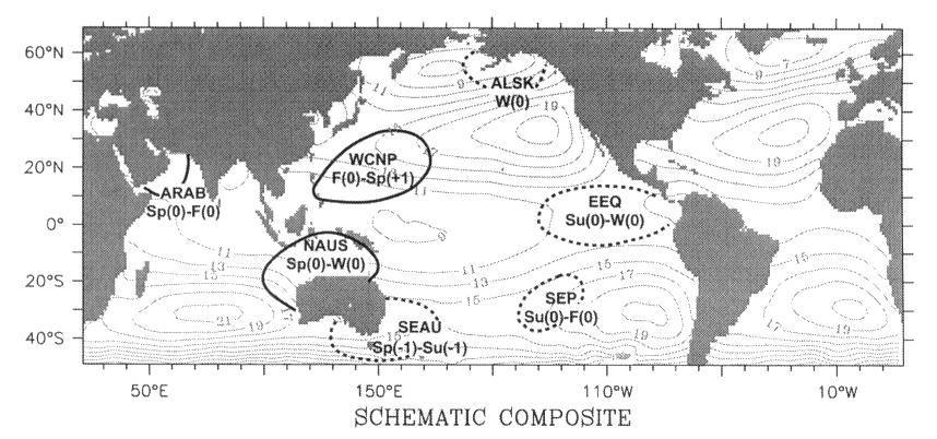
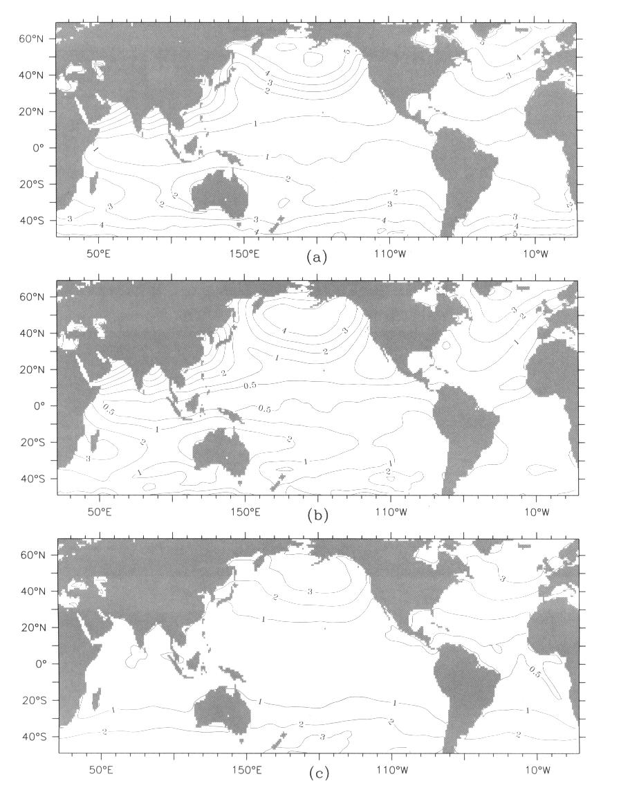
Fig. 7. Schematic representation of the major features of the composite, positive (solid line) and negative (broken line), superimposed on the annual mean SLP field. The boreal seasons for each feature are given, with Sp(-1) = March-April-May of Year(-1), etc. Contours are in (SLP - 1000) mb and the contour interval is 2 mb.
This schematic composite usefully summarizes the major features of the full composite, and illustrates that the global ENSO composite signal is not, fundamentally, a southern hemisphere event. In this respect the "Southern Oscillation" aspect of ENSO appears to have been over-emphasized. The northern hemisphere signal is both larger and more robust than the Southern Oscillation aspects of the signal.
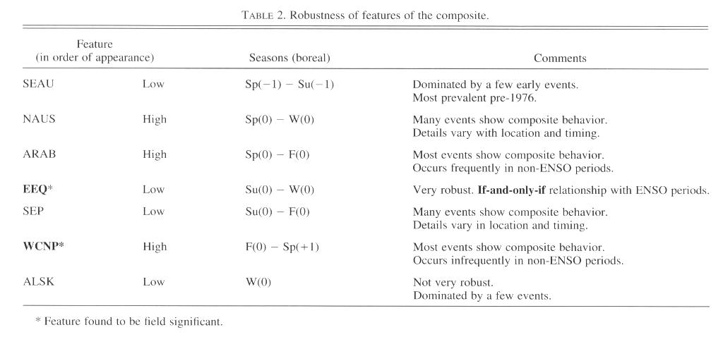
TABLE 2. Robustness of Features of the Composite
(Graphic image of table)
Feature |
Seasons (boreal) |
Comments |
|
| SEAU | Low | Sp(-1) - Su(-1) | Dominated by a few early events. Most prevalent pre-1976. |
| NAUS | High | Sp(0) - W(0) | Many events show composite
behavior. Details vary with location and timing. |
| ARAB | High | Sp(0) - F(0) | Most events show composite
behavior. Occurs frequently in non-ENSO periods. |
| EEQ * | Low | Su(0) - W(0) | Very robust. If-and-only-if
relationship with ENSO periods. |
| SEP | Low | Su(0) - F(0) | Many events show composite
behavior. Details vary in location and timing. |
| WCNP * | High | F(0) - Sp(+1) | Most events show composite
behavior. Occurs infrequently in non-ENSO periods. |
| ALSK | Low | W(0) | Not very robust. Dominated by a few events. |
* feature found to be field significant.
We have discussed all of the marginally significant features in this composite, but it is important to recall that only the EEQ and SEP lows and WCNP high features of the composite meet our significance criterion. The centers of these features do not show much zonal or meridional movement during the composite cycle. The EEQ trough forms quickly along the equator, deepens steadily for some months and then remains in place with nearly constant amplitude for several more months, until it shifts southward a few degrees as it weakens. The SEP trough forms in conjunction with EEQ but disappears quickly without moving. The WCNP ridge becomes more zonally oriented as it intensifies but shows little spatial change as it decays in Sp(+1).
To examine the robustness of these major features of our composite (that is, to determine the extent to which this behavior is present in every ENSO event, and only during ENSO events), as well as to see how representative the marginally significant features of the composite are, it is necessary to examine time series of SLPA over regions centered in the areas of these features. We do this in section 5.
Return to previous section or go to next section