Two types of gridded digital elevation models (DEMs) were developed for each study area; a DEM at medium resolution of 6 arc sec (∼180 m) for wave transformation from the open ocean to coastal areas; and a high resolution 1/3 arc sec (∼10 m) DEM for modeling of wave runup and inundation onto dry land. The grids for the forecast models and corresponding reference inundation model used by MOST model were sampled from these two DEMs.
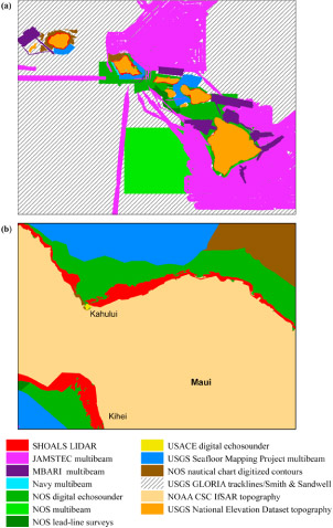
The DEMs were compiled from several data sources. For example, Figure 4 is an overview of the spatial extents of each data source incorporated into the medium-resolution and the high-resolution DEMs for Kahului. Table 2 is an overview of the data sources used; in general, the data sources listed first superseded data sources listed later in the area where they overlapped. All selected input data sets were converted to the mean high water (MHW) vertical datum, as necessary. Horizontal positions were reprojected, where necessary, to the WGS84 horizontal geodetic datum. Details are given by Tang et al. [2008b].
Fig. 4. Bathymetric and topographic data source overview. (a) Hawaiian Islands with 6 arc sec (∼180 m) resolution and (b) central Maui with 1/3 arc sec (∼10 m) resolution.
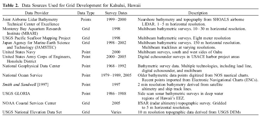
Table 2. Data sources used for grid development for Kahului, Hawaii.
How sensitive are the model outputs, including time series and inundation, to changes in the grid resolution, computational domains, accuracy of bathymetry/topography and other parameters? This issue is central to model development, because even with a correct tsunami source and a well-validated tsunami inundation numerical model, inappropriate model setup or inaccurate bathymetry/topography can produce poor or incorrect results.
Two case studies, at Kahului and Honolulu, were examined to evaluate the impact of model grid extent and resolution on the modeling results. For each tsunami, an identical tsunami source was applied to different model setups.
Figure 5a and Table 3 show how the changes of grid setup affect the model accuracy and speed at Kahului for the May 2006 Tonga tsunami. The grids for setups 1, 2 and 3 in Table 3, were derived from the same DEMs developed in 2005. Setups 1 and 2 are the first and revised Kahului forecast model. Setup 3 was the first Kahului reference inundation model. Prior to the 2006 Tonga tsunami, the forecast model setup 1 was tested with six past tsunamis, including the 2003 Rat Island, 2003 Hokkaido, 1996 Andreanof, 1994 Kuril Islands, 1964 Alaska and 1957 Andreanof tsunamis. Setup 1 produced good comparisons to these observations at Kahului tide station. The May 2006 Tonga event provided the first empirical test of the model with a wave propagating from the southwest. The incoming waves traveled through the shallow channels among the Maui Complex and exposed substantial deficiencies in the resolution and computational domain in the intermediate grid in setup 1. This illustrates the importance of testing tsunamis with all potential directionalities, especially for the Hawaiian Islands, which are in the middle of the Pacific Ocean. In 2007, nearshore bathymetric/topographic SHOALs airborne LIDAR with 1–5 m horizontal resolution from the Joint Airborne Lidar Bathymetry Technical Center of Expertise became available for Maui. Then the DEMs were updated and Kahului forecast and reference models were also redeveloped using the newest data source. More details on the updated models can be found at Tang et al. [2008b].
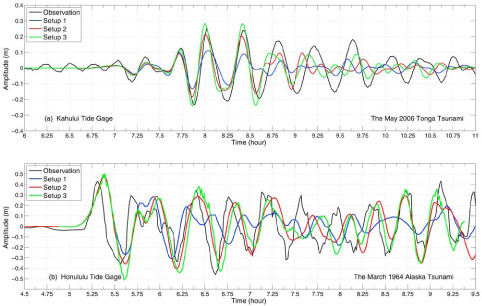
Fig. 5. Tsunami time series computed from different model setups at (a) Kahului tide gauge for the May 2006 Tonga tsunami and (b) Honolulu tide gauge for the March 1964 Alaska tsunami.
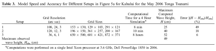
Table 3. Model speed and accuracy for different setups in Figure 5a for Kahului for the May 2006 Tonga Tsunami.
In Figure 5b, at Honolulu for the 1964 Alaska tsunami, grid setup 2, with a higher resolution, shows better comparison of wave height and phase for the later waves than those of setup 1. While model run time for a four hour simulation is less than ten minutes for setups 1 (120, 24, and 2 arc sec) and 2 (120, 18, and 2 arc sec), run time for the high-resolution setup 3 (36, 6 and 1/3 arc sec) is 64 hours. Finer resolution better resolves the individual structures of Honolulu harbor.
Tsunami forecast models for use in real-time operation need to balance between speed and accuracy. The models must complete within acceptable time limits, while using the highest resolution and largest computational domains possible. Currently, each forecast model is set up to run on a single processor in minutes. With the potential use of supercomputers in the future, the forecast speed can be further improved.
Accurate simulation of tsunami runup and inundation requires high quality runup and inundation data, high-resolution bathymetry and topography data in the runup area and good tsunami source parameters. Titov et al. [2005] have shown that, under these conditions, the MOST modeled runup and inundation agree quite well with survey data on Okushiri Island of the 12 July 1993 Hokkaido-Nansei-Oki Mw = 7.8 earthquake. At present, one major difficulty in inundation forecasting is a lack of high quality inundation/ runup measurements to verify the accuracy of topography and to calibrate the friction coefficient.
Topography/bathymetry compiled with incorrectly aligned datum or from different data sources can produce different inundation results. Figures 6a and 6b show the inundation computed from two sets of grids with the same 2 arc sec (∼60 m) resolution for the nearshore grids of Hilo forecast model for the 1946 Unimak tsunami. Grid 2 correctly reproduced the inundation limit as the measurements (Figure 6c), while no inundation was produced in grid 1 (Figure 6a). The topographic 0, 2, 5 and 10 m contours are quite different between these two grids. Developed in 2006 for the Hilo forecast model, all data sources for Grid 2 were converted to WGS 84 horizontal geodetic datum and mean high water vertical datum, when necessary. The data source for grid 1 was digitized and interpolated from the United States Geological Survey (USGS) maps.
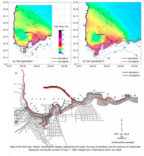
Fig. 6. (a and b) Maximum water elevations at Hilo computed from two sets of topographic and bathymetric grids for the April 1946 Unimak tsunami. (c) Comparison between computed inundation in Figure 6b and survey data from Shepard et al. [1950].
Figures 7a and 7b show how two topographic data sources produced different inundation results along the coastline from Ewa Beach to the Pearl Harbor entrance by a simulated TMw 9.3 tsunami from Solomon subduction zone near Santa Cruz Islands. Both nearshore grids have 1/3 arc sec (10 m) resolution. Recent high-resolution topographic LIDAR from the NOAA Coastal Services Center was applied in grid 2, which was developed for a tsunami hazard assessment study for Pearl Harbor [Tang et al., 2006]. The topographic data for grid 1 was derived from USGS 7.5 min DEM based on 30 m data spacing. The major 2, 5 and 10 m contours agree reasonably well for these two data sets. However, the topographic LIDAR data show a long narrow dune with an elevation around 2 m along Ewa Beach, which is absent in the USGS DEM. This explains the difference in inundation seen in Figure 7. Coastline with long narrow dunes is quite a common feature on the Hawaiian Islands. Attention must be paid to such features during grid development.
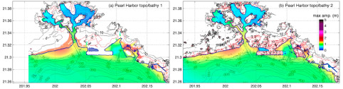
Fig. 7. Inundations at Pearl Harbor computed from two sets of topographic data sources used for a simulated TMw 9.3 tsunami. Topography was derived from (a) USGS DEM and (b) CSC LIDAR data. Color represents the maximum water elevation in m.
A smaller Manning coefficient can produce greater inundation over flat areas in some cases. However, the model can become unstable with a small Manning coefficient for certain large tsunami waves. Because of the model's sensitivity to the Manning coefficient, inundation extents may be subject to uncertainty in low-lying flat areas near the coast. The computed time series at a tide gauge location is generally less sensitive to the Manning coefficient setting. Figure 8 compares the inundation computed by the Kahului forecast model using different friction coefficients for two scenarios, (1) the April 1946 Unimak tsunami and (2) a simulated TMw 9.3 tsunami from Kamchatka. In Figure 8a, three different Manning coefficients, n = 0.01, 0.025 and 0.032, generate similar inundation lines for most of the coastline where the slope is relatively steep. However, the coefficient of 0.01 produces greater inundation in several flat areas such as the area southeast of Kahului Harbor. Figure 8b compares the inundation computed with n = 0.025 and 0.032 for the TMw 9.3 Kamchatka scenario. Though there are some minor differences at several locations, the inundation limit agrees well for this test case.
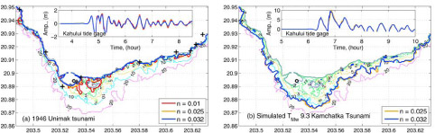
Fig. 8. Sensitivity of inundation and time series of tsunami amplitudes computed by the Kahului forecast model to Manning coefficients for (a) the April 1946 Unimak tsunami and (b) a simulated TMw 9.3 Kamchatka tsunami. Dots, Kahului tide gauge; crosses, Tsunami runup record from Pararas-Carayannis [1969].
The four forecast models in Hawaii and their corresponding higher resolution reference inundation models were tested with the fourteen historical tsunamis summarized in Table 1. Tide gauge data of the recent tsunamis, No.1 to 9, were from the NOAA National Water Level Observation Network (NWLON) [Allen et al., 2008], while others were digitized from Shepard et al. [1950], Zerbe [1953], Salsman [1959], Berkman and Symons [1964], and Spaeth and Berkman [1967]. The observations were filtered by a low-pass Butterworth filter with a cut-off of 60 or 120 min, to isolate lower-frequency components (including tide), which were then substracted from the raw data. In this section, we validate and evaluate the model performance through comparison of tsunami amplitude time series, period/frequency components via wavelet-derived spectra, and error estimation.
Figure 9 summarizes observed and modeled tsunami time series by the four forecast models at (1) Nawiliwili, (2) Honolulu, (3) Kahului, and (4) Hilo tide stations. When no observation is available, results from the forecast models were then compared with those computed by the higher resolution reference inundation models to ensure numerical consistency. The complete comparisons for each reference inundation model are documented in a technical report for each forecast site [Tang et al., 2008b, 2009].
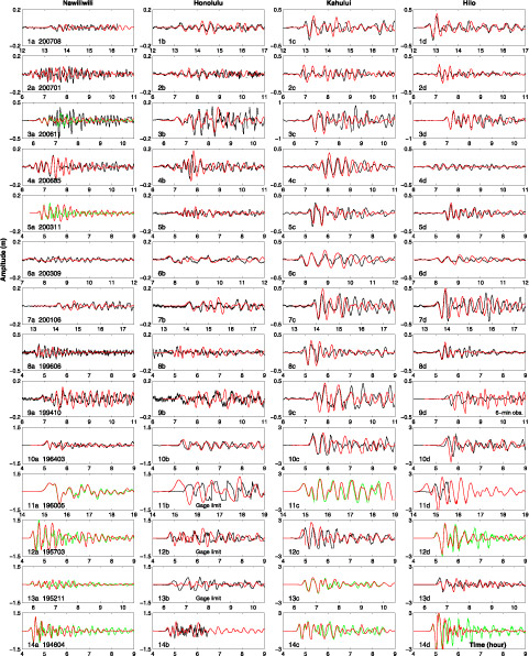
Fig. 9. Modeled and observed tsunami time series at Nawiliwili, Honolulu, Kahului, and Hilo tide stations for fourteen tsunamis. When no observation is available, results from the forecast models are compared with those from the reference inundation models. Black lines, observations; red lines, forecast models; green lines, reference inundation models. A 12 min adjustment was applied to the model time series 1a–1d for the August 2007 Peru tsunami.
Several recent tsunami events with a variety of geographic locations and source dynamics have provided rigorous tests of the forecast system. The most recent tested event is the 15 August 2007 Peru tsunami. A detailed description of the real-time experimental forecast for this tsunami is given by Wei et al. [2008]. At Hilo, Kahului, Honolulu and Nawiliwili tide stations, the observed maximum wave heights are 67, 56, 11 and 8 cm while the forecasts are 65, 55, 15 and 8 cm, respectively. As will be discussed in section 3.3, the forecasts showed earlier arrivals around 12 min. After this 12 min time difference was adjusted in Figure 9 time series 1a–1d, the forecasts and observations matched well in period.
The 13 January 2007 Kuril Islands earthquake occurred as normal faulting (USGS, M8.1 Kuril Islands earthquake of 13 January 2007, Earthquake Summary Map XXX, ftp://hazards.cr.usgs.gov/maps/sigeqs/20070113/ 20070113.pdf, 2007). The TMw 7.9 source was inverted from tsunami data recorded at three DARTs, 21414, 46413, and 21413, by a linear least squares fit to negative tsunami source functions near the epicenter. While it shows good comparisons at Nawiliwili and Honolulu, the maximum wave heights at Hilo and Kahului were overestimated (Figure 9 time series 2a–2d).
The Kuril Islands tsunami of 15 November 2006 provided ample tsunami data and the first test of NOAA's new experimental tsunami forecast system. The tsunami source was inverted with tsunami data recorded at several DART buoys along Aleutian Trench. The modeled first waves agree well with the observations, especially at Hilo and Honolulu (Figure 9 time series 3b and 3d). At Nawiliwili, the maximum wave height is underestimated (Figure 9 time series 3a). As will be discussed later, the discrepancy could also be contributed partially by nontsunami factors.
The 3 May 2006 Tonga earthquake generated a tsunami that was detected about six hours later by two offshore DARTs located to the south of the Hawaiian Islands. These data were combined with the TSF database to produce the tsunami source by inversion [Tang et al., 2008a]. Excellent agreement is obtained for the first 6 waves over 2 hours, including the amplitudes, arrival time and wave period (Figure 9 time series 4a–4d). The forecast models reproduced the maximum waves that arrived 1.5 hours since the first arrivals. Those are the 4th wave at the Hilo and Kahului stations, the 7th wave at Honolulu, and the 5th wave at Nawiliwili. As shown by Tang et al. [2008a], the Hilo and Kahului forecast models also modeled well the large amplitude later waves reflected from North America and scattered by South Pacific bottom features that reached the Hawaiian Islands 16 and 18.5 hours, respectively, after the earthquake.
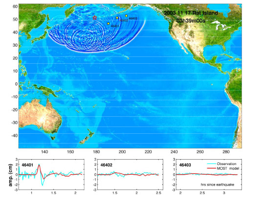
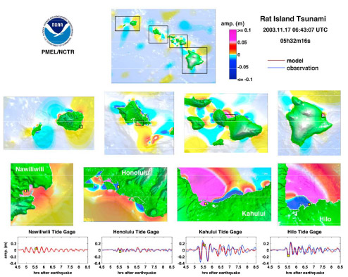
The 17 November 2003 Rat Islands tsunami provided the first real-time test of NOAA's forecast methodology, which became the proof of concept for the development of the tsunami forecast system [Titov et al., 2005]. This tsunami was detected by three DARTs located along the Aleutian Trench. The real-time data was combined with the TSF database to produce a tsunami source of TMw 7.8 by inversion. The offshore model scenario was then used as input for the Hilo forecast model, which was the first and the only forecast model under testing at that time. The grid resolutions were 120, 10 and 2 arc sec and the grid sizes were 196 × 161, 119 × 150, 125 × 170, respectively. The model runtime is about 10 min by using a single processor on a DELL PowerEdge 2650 with 2 Intel Xeon CPUs of 2.8 GHz, each with 512 KB cache and 4 GB memory. The accuracy of the forecast is reflected by the excellent agreement between the model prediction and observation at Hilo tide station (Figure 9 time series 5d). The forecasted maximum wave height at Hilo tide station is 0.43 m, while the observation is 0.45 m (−5% error); the error of the arrival time of the maximum wave is less than 1 min. It was the first time in history that the forecast of tsunami time series was available to a coastal city before tsunami waves arrived. The offshore forecasts of the maximum tsunami amplitude and arrival time are in Figure 1. Figures 2 and 3 show the maximum amplitude in the telescoping grids for the four forecast models and the Kahului reference inundation model, respectively. Figures 2 and 3 demonstrate, among other features, the dramatic change in tsunami scale from propagation to shoaling. The offshore amplitudes are small, about 1 cm at a water depth of 4000 m. Even when the water depth decreases to 50 m, the maximum amplitude is only about 8 cm. However, the amplitude increases dramatically due to shoaling when the tsunami waves enter a nearshore area shallower than 20 m and even more so because of local shelf and harbor resonances and other coastal effects. Similar behavior is observed for the May 2006 Tonga tsunami by Tang et al. [2008a]. This emphasizes the importance of high-resolution inundation models, which resolve the local coast and harbor geometries, in order to achieve accurate forecasting of tsunami amplitude nearshore; ocean-wide propagation models are insufficient. Movie S1 illustrates the progression of the tsunami propagation and the wavefront evolution affected by the near- and far-field bathymetric features. Movie S2 shows the tsunami waves near the coast of Hawaiian Islands.
Movie S1. Propagation of the 17 November 2003 Rat Islands Tsunami in the Pacific Ocean. Animation available in the HTML.
Movie S2. The 17 November 2003 Rat Islands Tsunami in Hawaiian Islands. Animation available in the HTML.
The 25 September 2003 Hokkaido earthquake generated tsunami waves of very long periods recorded at the Hawaiian tide stations. The wave amplitude decreased slowly and steadily (Figure 9 time series 6a–6d).
DART station 51406, located midway between South America and Hawaii, was not deployed until one month after the 23 June 2001 Peru tsunami. Therefore, the source for this event was derived based on an inversion of Kahului tide gauge records using the Kahului forecast model. In addition to Kahului, it produced good comparisons of first waves at the other three stations (Figure 9 time series 7a–7d).
Deep ocean research bottom pressure recorder data are also available for two other tsunamis. The inversion of the 1994 Kuril Islands tsunami data was done by using five BPR recordings while the 1996 Andreanov used one [Titov et al., 2005]. Model results agree quite well with observations for the first several waves (Figure 9 time series 8a–8d and 9a–9d). While other three stations recorded tsunami time series data at 1 min interval for the 1994 Kuril tsunami, only 6 min data are available at Hilo tide station. The 6 min resolution was unable to fully resolve the tsunami waves so the wave height at Hilo was under recorded (Figure 9 time series 9d).
DART buoy records are not available for the five destructive tsunamis, the 1964 Alaska, the 1960 Chile, the 1957 Andreanof, the 1952 Kamchatka and 1946 Unimak events. Previous studies of seismic, geodetic and water level data have estimated source parameters for some of the events [Green, 1946; Kanamori and Ciper, 1974; Johnson et al., 1994, 1996; Johnson and Satake, 1999; López and Okal, 2006]. However, some of the sources are subject to debate and adjustment. Most of the source estimates that have been done are based on low-resolution tsunami propagation models. The forecast system provides a unique chance to reinvestigate the historical sources by inversion of the water level data with the high-resolution quality inundation and propagation models. Preliminary results are available for the 1964, 1957, 1952 and 1946 tsunamis. The incomplete tide gauge records in Hawaii and the distance from the source to the developed forecast models in U.S. present a substantial challenging to reinvestigate the 1960 Chile tsunami. So the source parameters of the tsunami are taken from Kanamori and Ciper [1974] in this study. Model results are plotted in Figure 9 time series 10a–10d to 14a–14d, respectively. Honolulu tide station is the only station in Hawaii that recorded all of the five destructive tsunamis. However, the 1960, 1957 and 1952 tsunamis reached the gauge limit.
Figures 10a–10d show the error of the maximum wave height computed by the four forecast models for the historical tsunamis that have complete wave height records. When the observed maximum wave height is less than 0.5 m, the maximum computed error is less than 0.3 m. At small amplitudes, noise in the observed signals and numerical error in the model are large compared to the observations. When the maximum wave height is greater than 0.5 m, the error is within ±20%; this uncertainty can be attributed primarily to uncertainties in the tsunami source, model setup and bathymetry. Arrival time of the first wave peak in general agree well with the observations, with errors less than ±3% of the travel time. So far, the largest discrepancy between the modeled and observed first arrival time is 12 min for the 2007 Peru tsunami. However, with an earthquake epicenter 460 km to the northwest of the 2007 Peru earthquake, the 2001 Peru tsunami has only 3 min discrepancy in the arrival time. This 12 min arrival discrepancy is currently under investigation.
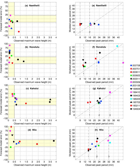
Fig. 10. (a–d) Error of the maximum wave height and (e–h) peak wave period from observations and model results by the Nawiliwili, Honolulu, Kahului, and Hilo forecast models. Forecast model error is (H − Hobs)/Hobs, where H is the modeled maximum wave height and Hobs is the observation. Colors represent subduction zones of the earthquakes. Red, central Kuril and Kamchatka; magenta, Hokkaido and west Kuril; black, Aleutian and Alaska; green, Tonga; blue, Peru; cyan, Chile.
Tsunami waves are known to produce time series with complex frequency structure that varies in space and time. To explore the tsunami frequency responses at different forecast sites, a complex Morlet wavelet transform was applied to both observations and model results. A description of the time series of wavelet-derived amplitude spectra is given by Tang et al. [2008a]. As an example, Figure 11 shows the real parts of the wavelet-derived amplitude spectra for the observation and the forecast at Hilo for the November 2006 Kuril Islands tsunami. The modulated spectrogram shows the first incident wave has a peak period near 20 min (Figure 11b). Quickly the tsunami excited two major oscillations with near 15 and 32 min periods in Hilo Harbor. Those changes of frequency structure were correctly captured by the forecast time series computed by the Hilo forecast model (Figure 11c).
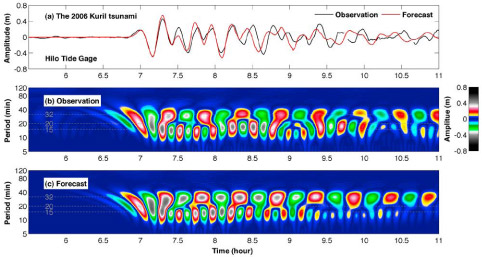
Fig. 11. (a) Time series of observed and forecast wave amplitudes at Hilo tide gauge computed by the Hilo forecast model in real time during the November 2006 Kuril Islands tsunami. Real parts of the wavelet-derived amplitude spectra of the (b) observed and (c) modeled tsunami waves are plotted.
The same approach was applied to the tsunami time series in Figure 9. Figures 10e–10h compare the observed and modeled peak wave periods at Nawiliwili, Honolulu, Kahului and Hilo. At Hilo, the observed peak wave periods fall into one of the three groups near 15, 22 or 32 min period (±2 min) (Figure 10h). The Hilo forecast model produced the peak wave periods reasonably well, especially in the highest frequency group (15 min period).
Similar to Hilo, at Kahului, the observed peak wave periods also fall into one of the three groups near 16, 24 or 32 min period (±2 min) (Figure 10g). The Kahului forecast model correctly reproduced the peak wave periods within groups 2 and 3. Although the modeled group 1 period does show up in the amplitude spectra for the 2006 and 2007 Kuril Islands tsunamis [Tang et al., 2008b], unlike the observations, it is not the dominant signal. The deep ocean tsunami observations at DART buoys for these two events show high frequency components appear in the later wave chains, which were not so well resolved in the propagation models. This may cause the peak period computed by the Kahului forecast model shifted from group 1 to group 2.
Honolulu Harbor has relatively complex geometry and tsunami waves can reach Honolulu tide station from both east and west harbor entrances. With relatively low signal-to-noise ratio data, Figure 10f shows wide range of the peak wave periods at the station. There are two distinct resonant oscillations near 11 and 22 min.
The relatively enclosed geometry of Nawiliwili Harbor produces a distinct, high natural frequency, making it different from the other three Hawaiian sites. The Nawiliwili forecast model produces the 16 min period well, and the 8 min period less well, leading to some uncertainty in forecasting such an event. The largest model-observation discrepancy in the maximum wave height was the 2006 Kuril Islands tsunami, with a 20 cm modeled maximum wave height for an 87 cm observation. The 1/3 arc sec (10 m) Nawiliwili reference inundation model produces a better fit with a 36 cm maximum height, yet still underestimates the later waves (Figure 9 time series 3a). Munger and Cheung [2008] also show large discrepancy between their maximum modeled and observed wave height at Nawiliwili for this event. Further investigation of this forecast site revealed the position of the tide station is right next to the cruise ship terminal where a ship, when docked, may affect the sensor. Coincidently, the Norwegian Star cruise ship started her docking procedures after the arrival of the first two small tsunami waves (delaying the scheduled arrival due to tsunami warning), potentially affecting the station recording. Although the exact effect of the ship interference with the tsunami signal has not been fully studied, the fact of additional data complexity at Nawiliwili is obvious.
Figures 10e–10h show that the peak wave period can be one of the local resonant periods. An interesting question is, for a particular tsunami, which local frequency may be excited as the peak frequency? Certain sites may have clearer clues than others. For example, at Kahului, Figure 10g indicates peak periods are related to the geographic locations of the earthquakes. Tsunamis originating from nearby subduction zone earthquakes excite similar peak periods at Kahului. Both the 2006 and 2007 Central Kuril Islands tsunamis have a peak period near 16 min (group 1), while the 1994 West Kuril Islands tsunami and the nearby 2003 Hokkaido tsunami present the same peak period near 32 min (group 3). The other seven tsunamis have similar peak wave periods near 24 min (group 2). Those are additional important information that can be useful for forecast and warning purposes.
To explore the hazardous wave conditions over the entire forecast site, maximum water elevation above MHW and maximum velocity computed by the forecast models were compared with those from the reference inundation models. Figures 2h and 3c show an example of Kahului for the 2003 Rat Island tsunami. Both the reference inundation model and the forecast model produced similar patterns and values. Comparisons for other tsunamis at Kahului are given by Tang et al. [2008b].
Model sensitivity studies and test applications in the previous sections provide lessons and guidance for developing site-specific tsunami models for use in operational forecasting. They have demonstrated that for a fixed tsunami source and a well-validated numerical tsunami inundation model:
Based on the above results, procedures and testing for development of tsunami forecast models are suggested as follows:
Derive DEMs from the best available bathymetric and topographic data sources at the time of development. Convert different data to the same vertical and horizontal datum. Update DEMs when better survey data becomes available.
Within acceptable computational time limits, apply the highest resolutions and largest computational domains for the forecast models. Develop a reference inundation model with highest possible resolutions and with extended computational domains for each forecast model to provide numerical references. Include bathymetric and topographic features within or close to the forecast site in the computational domains, such as nearby islands or long narrow dunes along coastlines, to provide correct coastal boundary conditions. Extend the regional grid to deep water to receive the correct dynamic boundary conditions from the coarse propagation scenarios.
Validate both the forecast model and reference inundation model with all available historical tsunami data for the model site, including tide gauge records and inundation/runup measurements. Test sensitivity of inundation to changes of friction coefficients.
Test forecast models and reference inundation models with different scenarios of simulated tsunamis based on major subduction zone earthquakes from all possible directions relative to the study sites. Verify the forecast model results with those of the reference inundation model to ensure numerical consistency. Test forecast models for stability for up to 24 hour model run for both historical and simulated scenarios of great subduction zone tsunamis.
Return to Previous section
Go to Next section