Natural fluctuations in climate dramatically influence biota in the Bering Sea (e.g., Napp and Hunt, 2001). Trends observed in 11 species (fish, marine birds, and marine mammals) found in the eastern Bering Sea/Aleutian Islands ecosystem show marked changes in relative abundance (Fig. 30.5). Using 100 physical and biological time series (29 of these from eastern Bering Sea marine biota), Hare and Mantua (2000) showed a significant change occurred in 1976/77 and to a lesser degree in 1989. While the mechanisms that link climate to biota were not addressed, it appears that a shift in the decadal patterns of climate (indicated by changes in the Pacific Decadal Oscillation and the Arctic Oscillation) contributed to changes in biota. More recently the change in the Pacific Decadal Oscillation (PDO) in the late 1990s has been interpreted as a regime shift (McFarlane et al., 2000; Macklin et al., 2002; Peterson and Schwing, 2003) or more recently as a shift in the dominate mode of variability in sea surface temperature (Bond et al., 2004). It is not necessary for the climate shift to be immediately manifest as biological change; shifts in the demersal fish communities are characterized by lags from the climate/ocean regime shift (Conners et al., 2002) and buildup of demersal fish stocks can exert top down control on populations of commercially important fish well after the climate shift (Bailey, 2000).
Figure 30.5: Schematic of ecosystem changes in the eastern Bering Sea showing trends of the relative abundance of select marine mammals, fish, and shellfish in the eastern Bering Sea (after NRC, 2003).
In the mid to late 1990s, the Eastern Bering Sea exhibited a host of noteworthy changes in physical and biological conditions (Kruse, 1998; Vance et al., 1998; Tynan, 1998; Baduini et al., 2001; Napp and Hunt, 2001; Hunt et al., 1999; Stabeno et al., 2001; Stabeno and Overland, 2001; Macklin et al., 2002; Napp et al., 2002; Olson and Strom, 2002): the first recorded major Bering Sea coccolithophorid blooms (1997, followed by blooms in 1998 through 2001), a large die-off of shearwaters (1997), salmon returns far below predictions (1997 and 1998), unusually warm summer sea surface temperatures (1997), unusually high ocean heat content (1998), and a decrease in the onshore transport of slope water (1997). While in the eastern Bering Sea, the abundance of pollock decreased (but continued to dominate biomass), a substantial increase occurred in gelatinous zooplankton (Brodeur et al., 1999a, 2002), arrowtooth flounder and other flatfish (Wilderbuer et al., 2002). Further, populations of Steller sea lions have continued their 30-year decline throughout the eastern Bering Sea. Below we address processes where the ocean temperature is directly related to sea ice processes and distribution, and to either wind or tidally generated turbulence and transport.
The pathways model (Fig. 30.2) considers sea ice as an important parameter, particularly fluctuations in extent, time of advance and subsequent melt-back, which are among the most striking physical phenomena (Schumacher and Stabeno, 1998) that also have profound impacts on biota (e.g., Hunt et al., 2002; Schumacher et al., 2003). Sea ice also provides habitat (e.g., haul outs) for some marine mammals, and once adequate solar radiation is available (early March), an under ice phytoplankton bloom occurs (Stabeno et al., 2001). The recent Oscillating Control Hypothesis (OCH; Hunt et al., 2002) relates climate change to energy flow and the timing of the plankton blooms, i.e., the timing of sea ice presence and melt-back is a critical aspect.
The interrelationships among the presence of sea ice, water column temperature, stability, and phytoplankton blooms (Fig. 30.6) have been observed from a long-term monitoring site on the middle shelf of the southeastern Bering Sea (Stabeno et al., 2001; Hunt et al., 2002). When ice is present in or after mid March, a strong peak occurs in chlorophyll fluorescence under the ice (e.g., 1995, 1997). The level of incoming short wave radiation prior to this time is likely insufficient to initiate a bloom of most phytoplankton species. The ice itself is relatively "thin" first year ice (<1 m) and has very little snow cover to attenuate or reflect incident radiation. When there is no ice present at this monitoring site (e.g., 2001), or the ice retreats before mid March (e.g., 1998, 2000), the bloom occurs in May or June. In 1999, sea ice was present at the site in late March, and returned in early May. As a result, there was an initial bloom in late March and another weaker and prolonged period of elevated fluorescence in late May and June.
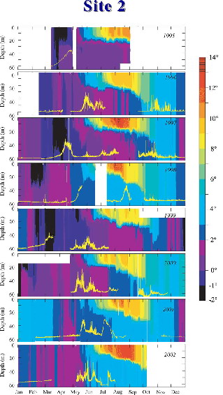
Figure 30.6: Time series of temperature contours at the long-term monitoring site in the middle domain (Site 2). Areas of black indicate cold water resulting from the presence of melting sea ice. The yellow line near the bottom of each panel indicates fluorescence at 11–13 m depth. For each year, the fluorometer tracts have been scaled to the highest value in that year. Gaps in this record occur due to fouling of the instrument or loss of mooring. (After Stabeno and Hunt, 2002.)
The spring bloom of phytoplankton associated with the sea ice accounts for 10–65% of the total annual primary production (Niebauer et al., 1995). A large proportion of the primary production from the sea-ice associated bloom eventually falls, unused, to the sea floor. This occurs because cold temperatures likely impact the ability of micro- and mesozooplankton grazers to effectively utilize the increase in production. Estimated total zooplankton production in 1999, a cold year, was 8–52% that of the two previous years when winter temperatures were average to above average (Coyle and Pinchuk, 2002a). While the total zooplankton production is dominated by small species that respond positively to temperature, at least one key species over the middle domain (Calayus marshallae) has higher standing stocks in colder years (Baier and Napp, 2003). In years when sea ice either does not exist over the southeastern shelf or retreats prior to the time when adequate light exists for a bloom (mid March), the spring bloom is delayed until later in the season when thermal stratification of the water column occurs (Stabeno et al., 2001). Under this scenario, phytoplankton biomass accumulates in the water column, but a much larger fraction of the primary production is utilized by zooplankton. The frequency of alternation between cold and warm regimes and the lengths of the individual stanzas may determine whether higher trophic levels are predominantly controlled by bottom-up or top-down mechanisms (Hunt et al., 2002; Hunt and Stabeno, 2002). In addition to how ice effects bottom up control of energy flow in the pelagic ecosystem, ice and its attendant cold pool directly influence the spatial distributions of higher trophic level biota (Ohtani and Azumaya, 1995; Wyllie-Echeverria and Ohtani, 1999; Brodeur et al., 1999b). As previously mentioned, avoidance of the cold pool often has the affect of increasing predation and cannibalism on larval and juvenile fishes by increasing the spatial overlap (or separation) of predator and prey.
In the Bering Sea, wind stress is another important physical force that strongly influences biological production as well as the flux of heat and nutrients (Fig. 30.2). Wind mixing largely determines the timing of the spring phytoplankton bloom when ice is not present, and helps to set annual new production through controlling the resupply of nitrate into the euphotic zone during summer (Sambrotto et al., 1986). Over the southeast shelf, the effect of wind mixing (through changes in water column stability) on nitrate uptake (primary production) can either decrease uptake during the respiration-limited phase or increase nitrate uptake once nutrients are limiting through resupply from deeper waters (Sambrotto et al., 1986). Not included in the pathway model are tides that strongly influence the southeastern Bering Sea. These two sources of turbulence are important to the region's biology and sediment processes.
The Inner Front Study, which began in 1997, focused on the importance of physical processes of the inner front to prolonged primary production. Results from Kachel et al. (2002) not only enhanced our knowledge of the inner front's physical characteristics, but they also elucidated some of its biological importance. During summer, nutrients could be pumped into the euphotic zone at the front, thereby stimulating production. The effectiveness of this process depends on two factors. First, a deep (sub-pycnocline) reservoir of nutrients must exist, and this is usually found within the middle shelf's bottom layer, the cold/cool pool. Typically, high concentrations of nutrients exist in the bottom layer over the middle shelf. An exception was 1997, when two factors (late spring storm and a shallow summer mixed layer) conspired to deplete nutrients from the cold pool. The strong, late spring storm vertically mixed the water column to a depth >50 m. Since nutrients in the euphotic zone had been depleted by an earlier, ice-associated, phytoplankton bloom, this caused the nutrient concentration in the cold pool to be reduced by almost half. Next, the very shallow mixed layer during the summer, allowed a phytoplankton bloom to occur beneath the surface mixed layer, which slowly consumed the nutrients in the cold pool (Stabeno et al., 2001; Stockwell et al., 2001). In addition to nutrients being available, sufficient mixing energy must occur to erode the extant vertical stratification. This can happen either by intensification of wind mixing and/or tidal mixing (throughout the fortnightly cycle); both of these processes move the inner front seaward. When this occurs, nutrients are made available to the frontal region, and are mixed upward where they can be utilized by phytoplankton. An example of this process can be seen in temperature and nitrate data collected across the inner front (Fig. 30.7). High concentrations occur within the cold/cool pool while those in the upper layer of the middle shelf and in the coastal domain are low. At the inner front, vertical finger-like structures with elevated concentrations of nitrate coincide with the 5.5°C isotherm. This structure was observed several days after an intense (wind speeds >14 m s![]() ) storm passed through the region and tidal currents were near their fortnightly maxima (Kachel et al., 2002).
) storm passed through the region and tidal currents were near their fortnightly maxima (Kachel et al., 2002).
Figure 30.7: Contours of temperature (color; .C) and nitrate (black lines; mmoles l.1). The locations of the CTD stations are marked along the bottom axis. Nutrients were measured on each cast. (From Kachel et al., in 2002)
Turbulence also can directly affect the efficiency of larval feeding. Megrey and Hinckley (2001) used a process-oriented individual based model (IBM) of larval pollock that incorporated a turbulence-contact rate-feeding success mechanism, thus relating wind generated turbulence to feeding. Output from the model agreed with hydrodynamic theory, with a well-defined peak in consumption at intermediate wind speeds (MacKenzie et al., 1994). The functional form of wind speed versus maximum consumption was determined by a quadratic fit to model results. Optimum feeding (540 μg dry weight per day per individual) occurred at a wind speed of ~7 m s![]() . At wind speeds >9.5 m s
. At wind speeds >9.5 m s![]() increased turbulence negatively affected feeding, and at wind speeds <4.8 m s
increased turbulence negatively affected feeding, and at wind speeds <4.8 m s![]() feeding was less than optimal because turbulence was not sufficient to enhance contact rate. Fish and plankton can regulate their exposure to turbulence by adjusting their vertical position in the water column (Incze et al., 2001; Olla and Davis, 1990). In the Gulf of Alaska, survival of larval pollock cohorts has been tied to coincidence of the critical first feeding period and calm weather (Bailey and Macklin, 1994).
feeding was less than optimal because turbulence was not sufficient to enhance contact rate. Fish and plankton can regulate their exposure to turbulence by adjusting their vertical position in the water column (Incze et al., 2001; Olla and Davis, 1990). In the Gulf of Alaska, survival of larval pollock cohorts has been tied to coincidence of the critical first feeding period and calm weather (Bailey and Macklin, 1994).
Transport, which is indicated in the pathway model as changes in horizontal flow, is critical to many aspects of ecosystem dynamics, including advection of nutrients and plankton. Several studies suggest a connection between changes in climate and changes in recruitment of fish and shellfish species (e.g., Incze et al., 1987; Rosenkranz et al., 2001;Wilderbuer et al., 2002). One mechanism often cited is a change in the direction of transport of the planktonic stages (towards or away from favorable habitat or predators). Wespestad et al. (2000) related changes in climate and their regional impact on wind fields and transport of larval pollock in an attempt to identify sources of recruitment variability.
Recent studies have shown this shelf has considerable north-south variability. The southeastern shelf contains three distinct regions or latitudinal zones along the 70-m isobath: a strong two-layered system with cold/cool pool that lies south of about 57°N, an intermediate zone consisting of more well-mixed water; and a two-layered system with the northern cold pool that extends northward from about 58°N (Stabeno et al., 2002). In the bottom layer over the middle shelf, distributions of salinity and nutrients (nitrate) appear correlated. The greatest salinities and nitrate concentrations occurred in the northernmost zone and may represent the impact of across-shelf transport due to the mean flow in this region (Reed, 1998). Slope/outer shelf domain plankton taxa have been observed near the inner front as further evidence of this cross-shelf transport (Coyle and Pinchuk, 2002b).
Transport has important ramifications for dissolved and planktonic material, including larval fish (Wespestad et al., 2000; Wilderbuer et al., 2002) and crabs (Rosenkranz et al., 2001). Wespestad et al. (2000) used a simple wind drift model to generate trajectories of pollock eggs and larvae over the southeastern shelf. After a time period related to larval development, the young pollock were subjected to cannibalism by age-2 and older adults. While this approach was consistent with some year-classes of high recruitment, it did not fit the recruitment every year. One caveat is that the wind drift model only applies to the upper few meters of the water column, and both pollock eggs (Kendall, 2001) and larvae exist deeper in the water column (Napp et al., 2000). In addition, using a single initial point for the eggs/larvae is an oversimplification of the actual spawning regions for pollock (Hinckley, 1987).
To address these disparities, a different transport model was used to simulate transport. The North-eastern Pacific Regional Ocean Model System (NEPROMS) was selected to simulate drifter trajectories that more closely simulate pollock egg and larval transport (D. Ridgi, personal communications). The simulated pollock eggs were initialized in a grid, which contained the initial point used by Wespestad et al. (2000), but the drifter initial positions are denser near the surface, replicating egg distribution data collected in the Bering Sea (Kendall, 2001). A prominent feature in this region (north and east of Unimak Pass) is the confluence of flow of the Alaska Coastal Current into the Bering Sea through Unimak Pass and the upslope flow of the ANSC in Bering Canyon (Stabeno et al., 2002). The initial drifter positions were a seven by seven grid with horizontal separations of about 10 km at the confluence of two flows. Vertically, there were 15 drifters initialized at each grid point to a maximum depth just over 40 m. Drifters were released on April 1 of each year and tracked for 90 days.
Simulations were conducted for the period 1997–2001. In all years there was a tendency for drifters to move either toward the northeast along the Alaska Peninsula, or toward the northwest along the 100 m isobath. This result is in agreement with a schematic of mean circulation (Fig. 30.4) and satellite tracked drifter trajectories (Schumacher and Stabeno, 1998). Recently, abundances of age-0 pollock in and around the inner front at Cape Newenham were estimated to be the same order of magnitude as those around the Pribilof Islands (Coyle and Pinchuk, 2002b). Model trajectories of drifters from 1997 show that a subset of the drifters that began by following the 100 m isobath and then veered to the northeast. In 2000, trajectories revealed a strong turning to the northwest of trajectories that had been moving along the Alaska Peninsula. Fig. 30.8 shows trajectories for 2001. The simulations also suggest the importance of interannual variations in transport. They also suggest how dependent the end points of the "larval drift" are to small variations in both horizontal (order 10 km) and vertical (order 5–10 m) initial positions. Numerous trajectories generated by a model, which includes only wind drift (OSCURS: Wespestad et al., 2000) were toward the northeast along the Alaskan Peninsula, as were the majority of the NEPROMS simulations in the upper five divergence of the trajectories. In the 5–20 m and 20–40 m release bins there were many drifters that followed the 100 m isobath to the northwest, with some even moving through Unimak Pass into the North Pacific Ocean before turning back. Further examination is required to determine the environmental parameters that resulted in the interannual differences in trajectories, and therefore to help understand how transport affects year class strength of pollock and other plankton.
Figure 30.8: Trajectories simulated for a 90-day period starting on 1 April 2001. The upper left panel shows all drifters, while the other panels show drifters divided as a function of initial release depth. Note that with increasing depth there is a greater tendency for drifters to flow northwestward and even become involved in the eddy-like circulation associated with the Bering Slope Current. This suggests a mechanism for planktonic transport between oceanic and shelf waters.