
We focus here on the effects of 1990s to 2000s warming of abyssal waters globally and deep waters in the Southern Ocean on heat gain and SLR. First, given the observed dθ/dt within a given depth range in each basin, we estimate the local heat flux required across the top of that depth range in each basin to account for that change and the local SLR implied by that change in each basin (section 4a). Second, we make a global estimate of the heat flux required to account for the sum of changes in individual basins and given depth ranges expressed as if the heating were distributed evenly over the entire surface of the earth (a climate literature convention) and, similarly, a global estimate of SLR expressed as a uniform change in height of the entire ocean surface (section 4b).
In many of the basins north of the SAF, warming trends on pressure levels become significantly different from zero at 97.5% confidence below around 4000 m, making this depth a natural division for this study. In many of the repeat sections within the Southern Ocean consistently strong warming extends higher in the water column south of the SAF. Hence, we also analyze contributions to SLR and heat gain from warming found from 1000 to 4000 m south of the SAF. We sum the changes found in these two regions (1000–4000 m south of the SAF and below 4000 m everywhere but the Arctic Ocean and Nordic seas). Both of these regions are primarily ventilated by AABW (Fig. 1; Johnson 2008), so our estimates may be loosely thought of as quantifying the effects of changes in AABW on local and global heat and sea level budgets, although other Southern Ocean changes likely also play a role, as discussed in section 5.
To calculate the local contribution of warming in each basin below 4000 m to the heat budget, dθ/dt estimates are converted to a heat flux ( Qi ) through the 4000-m isobath of each basin using
where a is the surface area of each depth, z, calculated using a satellite bathymetric dataset (Smith and Sandwell 1997). Prior to this integration, the dθ/dt profiles are interpolated from a pressure grid onto an evenly spaced 20-m depth grid for each basin. Profiles of density ρ and heat capacity Cp are estimated from climatological data (Gouretski and Koltermann 2004) for each basin using the mean temperature and salinity at each depth within that basin. The integral in (1) gives the total heating rate below 4000 m in each basin. Dividing by the surface area of the basin in question at 4000 m, a(4000), converts the total heating rate into a flux required through the 4000-m level in that basin to account for the observed warming beneath that level in that basin (Fig. 8a).
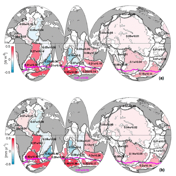
Fig. 8. (a) Mean local heat fluxes through 4000 m implied by abyssal warming below 4000 m from the 1990s to the 2000s within each of the 24 sampled basins (black numbers and color bar) with 95% confidence intervals. The local contribution to the heat flux through 1000 m south of the SAF (magenta line) implied by deep Southern Ocean warming from 1000 to 4000 m is also given (magenta number) with its 95% confidence interval. (b) Similarly, basin means of sea level rise from the 1990s to the 2000s due to abyssal thermal expansion below 4000 m and deep thermal expansion in the Southern Ocean from 1000 to 4000 m south of the SAF. Basin boundaries (thick gray lines) and 4000-m isobath (thin black lines) are also shown.
We find the 95% confidence interval associated with the Q for each basin using the volume-weighted variance of Q and volume-weighted DOF for that basin. The variance (standard deviation squared) of dθ/dt at each pressure in each basin is converted to a heating rate variance by multiplying by the square of ρCp. Then, the volume-weighted means for the variance and DOF below 4000 m are found using the a at each depth for a weight in the vertical integration. The standard deviation is then found by taking the square root of the variance and again the 95% confidence interval estimated assuming a Student's t distribution (Fig. 8a).
Similarly, we calculate the local SLR due to thermal expansion of each basin below 4000 m Fi using

where α is the thermal expansion coefficient. The associated 95% confidence intervals for each Fi are estimated following a method analogous to that described above for the local heat budget estimates (Fig. 8b).
The geographical distributions of local basin-mean warming and cooling below 4000 m from the 1990s to the 2000s (Fig. 8a) and closely associated SLR changes (Fig. 8b) reveal a clear global pattern. Of the 24 basins with data below 4000 m, 17 warmed (nine significantly different from zero at 97.5% confidence) and 7 cooled (one significantly different from zero at 97.5% confidence).
In general, a clear pattern in the magnitude of abyssal heating is seen: smaller values farther to the north and larger values to the south (Fig. 8). The three southernmost basins—the Weddell–Enderby, the Australian–Antarctic, and the Amundsen–Bellingshausen—show strong local warming below 4000 dbar of 0.33 (±0.28), 0.25 (±0.14), and 0.15 (±0.11) W m−2, respectively, all significantly different from zero at 97.5% confidence. We can trace the propagation of AABW from these southernmost basins northward and, with it, a waning warming (or cooling) signal. In each of the three oceans, AABW flows generally north from basin to basin, subject to bathymetric constraints. However, the Atlantic, Indian, and Pacific oceans each present a slightly different pattern that should be viewed with the AABW flow in mind, as discussed below.
In the Atlantic Ocean, the warming pattern follows the flow of AABW out of the Southern Ocean. AABW leaves the Weddell Sea across the South Scotia Ridge and through the Sandwich Trench, traveling toward the western North Atlantic through the Argentine and Brazil basins in the western South Atlantic (Coles et al. 1996; Orsi et al. 1999; Jullion et al. 2010). The Argentine and Brazil basins, containing mostly AABW in the abyss (Fig. 1a; Johnson 2008), show warming, with that of the latter being statistically significant. The abyssal western North Atlantic, which contains little AABW influence, shows only a small amount of warming, not significantly different from zero (Fig. 8). At the equator, deep and bottom waters cross into the Angola Basin and travel north and south, filling the basins east of the Mid-Atlantic Ridge through deep passages (Warren and Speer 1991). These eastern Atlantic basins all show abyssal cooling with the northernmost basin being the only one showing statistically significant cooling in this study. However, the dominant abyssal influence in these eastern basins is NADW, not AABW (Fig. 1; Johnson 2008). On the other hand, the strong and statistically significant recent warming in the deep Caribbean Sea, filled with NADW that spills over a relatively shallow ∼1800-m sill, is part of a trend starting a few decades prior to the 1990s (Johnson and Purkey 2009).
In the Indian Ocean both warming and cooling basins are found (Fig. 8). Basins to the west of the Ninetyeast Ridge mostly show deep cooling, although none of these basins exhibits cooling significantly different from zero at 97.5% confidence, while the two basins to the east of the ridge show statistically significant warming. Two of the basins west of the Ninetyeast Ridge, the Somali Basin and Arabian Sea, are not sampled. Since the deepest sills of these basins connect them to adjacent basins exhibiting cooling, one could speculate that these unsampled basins might have shown cooling had they been sampled repeatedly, although the adjacent cooling is not statistically different from zero at 97.5% confidence. As in the Atlantic, the magnitude of the warming (or cooling) in the Indian Ocean basins decreases with distance from the Southern Ocean. The warming Agulhas–Mozambique Basin, located directly south of Africa between the cooling Cape Basin in the southeast Atlantic Ocean and the cooling Crozet and Madagascar Basins in the southwest Indian Ocean, stands out as an anomaly to this pattern. Data from two tracklines crossing the dynamic Agulhas–Mozambique Basin were used in this calculation (Fig. 1a): I05 shows uniform cooling across the northeast region of the basin, but I06 alternates between warming and cooling while crossing the fronts of the ACC. Hence, these data estimate overall warming in the basin, but with a large uncertainty.
In contrast to the Atlantic and Indian oceans, the Pacific Ocean (Fig. 8) exhibits deep warming that is significantly different from zero at 97.5% confidence in its large central basins with more uncertain warming in most of its small peripheral basins. One of the peripheral basins shows very slight (0.01 W m−2) but statistically insignificant cooling. Similar to the other two oceans, the magnitude of the warming in the Pacific basins decreases northward from the Southern Ocean.
To complement the local estimates of warming and SLR below 4000 m, Q and F are calculated for the region between 1000 and 4000 min the Southern Ocean south of the SAF, where AABW influence is also strong (Fig. 1b; Johnson 2008). Equations (1) and (2) are applied following the same procedure as described above but using the area and dθ/dt from the Southern Ocean. The heating between 1000 and 4000 m in the region contributes an additional 0.91 (±0.82)W m−2 and 0.87 (±0.76) mm yr−1 to the local heat flux and SLR, respectively. Adding these local changes to the heat flux and SLR below 4000 m in the Southern Ocean yields local heat gains equivalent to a local heat flux on the order of 1 W m−2 and SLR on the order of 1 mm yr−1.
The observed local heat flux and SLR are combined in rough estimates of the recent abyssal and deep Southern Ocean warming's contributions to global heat and SLR budgets. The total heat flux and error at each depth can be calculated by summing the results fromall basins using

and the 95% confidence interval on that sum estimated using

where SAearth is the total surface area of the earth and the subscript b denotes each basin (Fig. 9a). The global heat flux is expressed in terms of an application to the total surface of the earth, as is customary for global energy budget studies, rather than the surface area of the ocean.
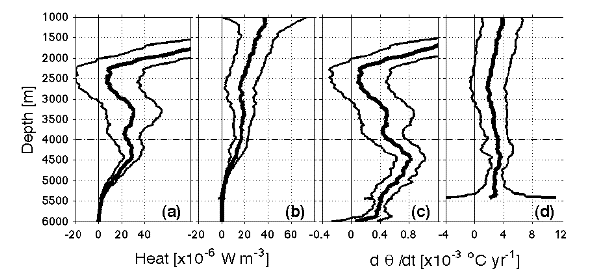
Fig. 9. Profiles of heat gain per meter (thick lines) with 95% confidence intervals (thin lines) estimated as described in (3) for the (a) global ocean and (b) Southern Ocean south of the SAF. Area-weighted mean profiles of dθ/dt for (c) the global ocean and (d) the Southern Ocean south of the SAF.
The factor of 2 in (4) yields a conservative estimate for the 95% confidence limits from a Student's t distribution. The DOF of the 24 sampled basins ranges from 4 to 283 with a mean and median of 37 and 23, respectively. The estimate in each basin is independent, making the DOF easily greater than 60, thus this factor could arguably be slightly less than 2. The eight basins that were not sampled are assumed to have a zero warming rate.
The contribution of the Southern Ocean Q (Fig. 9b) to the global heat budget can be derived by dividing by SAearth instead of the basin surface area in (1). Again, we express this contribution as a uniform heat flux applied to the entire surface area of the earth. Comparing the global heat flux (Fig. 9a) to the heat flux south of the SAF (Fig. 9b) further emphasizes the result (Fig. 8) that the abyssal temperature changes contribute a statistically significant fraction of the observed global change in addition to the deep Southern Ocean warming. Above 4000 m almost all of the deep warming can be accounted for by warming in the Southern Ocean, again supporting the choice made here of focusing on global abyssal changes below 4000 m and Southern Ocean deep changes from 1000 to 4000 m.
Area-weighted mean dθ/dt profiles for the global and Southern oceans (Figs. 9c,d) emphasize that the deep warming rate in the Southern Ocean is much larger than that in the global ocean. Also, warming temperature trends remain strong to the bottom; contributions of abyssal warming to the heat budget decrease with increasing depth primarily because the area of the ocean decreases with increasing depth.
We make an estimate of the total heat gain from recent deep Southern Ocean and global abyssal warming by adding the integral of Qabyssal below 4000 m to the integral of QSouthernOcean from 1000 to 4000 m (Table 1). The 95% confidence interval for Qabyssal is calculated as the square root of the sum of the basin standard errors squared times 2, again using this factor because the DOF exceed 60. The warming below 4000 m is found to contribute 0.027 (±0.009) W m−2. The Southern Ocean between 1000 and 4000 m contributes an additional 0.068 (±0.062) W m−2, for a total of 0.095 (±0.062) W m−2 to the global heat budget (Table 1). Following the same procedure, the contribution of these warmings to SLR due to thermal expansion can be estimated using α instead of ρCp and the surface area of the ocean instead of the surface area of the earth. A global contribution of 0.145 (±0.083) mm yr−1 of SLR can be linked to this thermal expansion (Table 1).
The above calculations assume that the unsampled basins give zero contribution to the heat budget. We investigate the effects of two alternative scenarios on the estimates. For the first scenario, we assume that the unsampled basins have a dθ/dt profile equal to the mean dθ/dt profile of all the sampled basins. This scenario increases our global abyssal estimate by 0.0006 W m−2. For the second scenario, we assume that the unsampled basins have a dθ/dt profile identical to that of the adjacent basin with the deepest connecting sill upstream in terms of abyssal flow, where the abyssal water supplying the basin in question likely originated. The two unsampled deep basins in the Indian Ocean—the Somali Basin and Arabian Sea—are assumed to be connected to the Madagascar Basin and mid-Indian Basin, respectively. In addition, dθ/dt of the central Pacific basin is used for the Sea of Okhotsk, Sea of Japan, and the Coral Sea, and dθ/dt of the Peru Basin is used for the Guatemala and Panama Basins. However, as mentioned earlier, all of these basins are either completely or mostly shallower than 4000 m; therefore, they have little impact on the estimates given here. The scenario decreases the global mean estimate of deep Southern Ocean and global abyssal heat gain by 0.0009 W m−2. Thus, for either of these methods of accounting for the unsampled basins, the global values remain identical at the quoted precision (Table 1).
In addition to using 4000 m as the shallower limit for the global abyssal estimate and the deeper limit for the deep Southern Ocean estimate of warming, we also present global heat flux and SLR estimates using 3000 and 2000 m for that dividing depth (Table 1). We believe that 4000 m is the more appropriate choice for quantifying primarily the effects of AABW warming. However, since the deepest known studies of ocean heat uptake of which we are aware extend only to 3000 m (Levitus et al. 2005) and the Argo array allows estimates to 2000 m since about 2003 (e.g., von Schuckmann et al. 2009), we calculate the global flux and SLR below 3000 and 2000 m for comparison with these works. The 2000-m numbers should be used with caution. Above 3000 m, changes along a given section may be influenced by changes in the wind-driven circulation (e.g., Roemmich et al. 2007), requiring better temporal and spatial sampling than available from repeat hydrography to quantify properly. Thus, we may be underestimating uncertainties above 3000 m since we may be aliasing wind-driven processes that are not captured by the spatially sparse and decadal sampling scheme.
When 3000 m is used instead of 4000 m, the same local basin patterns emerge (not shown). The only basin where the mean changes sign is the South Fiji Basin,which trends from warming at 0.00 W m−2 to cooling at 0.02 W m−2. The error-to-signal ratio for local heating rates below 3000 m increases substantially in many of the basins compared with that below 4000 m, with none of the basins' cooling being statistically significant. Using a 2000-m interface depth gives an even higher abyssal heat flux (not shown), also with an even higher error-to-signal ratio.
Again, following (3) and (4), the recent decadal global heat gain in the deep ocean can be estimated by adding Qabyssal below 3000 (or 2000) m to the QSouthernOcean between 1000 and 3000 (or 2000) m (Table 1). As expected, using this 3000-m interface the global contribution below 3000 m increases compared to that below 4000 m. The Southern Ocean contribution, between 1000 and 3000 m is less than between 1000 and 4000 m. The sum, however, is roughly the same. Similarly, using the 2000-m interface depth raises the global contribution but lowers the Southern Ocean contribution with the sum remaining roughly the same. Again, these similarities exist because most of the observed warming between 2000 and 4000 m is located in the Southern Ocean (Fig. 9), and therefore choosing 4000, 3000, or 2000 m does not change the heat gained by the ocean below that interface north of the SAF. However, the partition of error associated with the estimates shifts as the interface depth is changed. The abyssal contribution has a signal 3.2 times its 95% confidence with the 4000-m interface, but only 1.7 (1.1) times its confidence using 3000 (2000) m because the bottom-intensified abyssal warming signal is most robust near the bottom.
Return to Abstract
Return to Previous section
Go to Next section