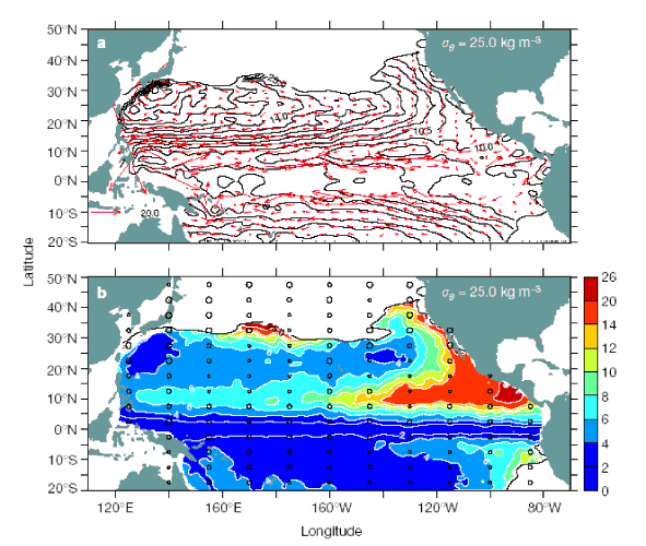
Figure 1. Mean circulation and potential vorticity averaged over 50 years
(1950–99) in the upper pycnocline of the Pacific Ocean. a, Geostrophic
streamlines relative to 900 dbar (in m![]() s
s![]() )
and b, absolute value of potential vorticity (in 10
)
and b, absolute value of potential vorticity (in 10![]() m
m![]() s
s![]() )
on the 25.0 kg m
)
on the 25.0 kg m![]() potential
density surface. Velocity vectors are overplotted on a. Distribution of hydrocasts
down to 900 dbar is overplotted on b, with the size of the dots representing
total number of casts in regions of 5° latitude by 15° longitude
(smallest, 50–300; intermediate, 301–1,000; largest, 1,001 or more).
Winter season outcrop lines are drawn in both panels. The outcrop lines define
locations where wintertime surface mixing penetrates deepest into the pycnocline,
creating new water masses that are subsequently sequestered from the atmosphere
as seasonal heating restratifies the upper ocean in spring and summer. Potential
vorticity is defined as f(
potential
density surface. Velocity vectors are overplotted on a. Distribution of hydrocasts
down to 900 dbar is overplotted on b, with the size of the dots representing
total number of casts in regions of 5° latitude by 15° longitude
(smallest, 50–300; intermediate, 301–1,000; largest, 1,001 or more).
Winter season outcrop lines are drawn in both panels. The outcrop lines define
locations where wintertime surface mixing penetrates deepest into the pycnocline,
creating new water masses that are subsequently sequestered from the atmosphere
as seasonal heating restratifies the upper ocean in spring and summer. Potential
vorticity is defined as f(![]()
![]() /
/![]() z)/
z)/![]()
![]() ,
where f is the Coriolis parameter,
,
where f is the Coriolis parameter, ![]()
![]() /
/![]() z
is the vertical density gradient, and
z
is the vertical density gradient, and ![]()
![]() is
a constant reference density (10
is
a constant reference density (10![]() kg
m
kg
m![]() ).
Water parcels conserve
their potential vorticity in an ideal fluid.
).
Water parcels conserve
their potential vorticity in an ideal fluid.
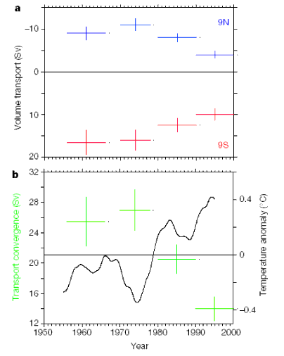
Figure 2. Meridional transports in the pycnocline and smoothed sea surface
temperatures over the past 50 years. a, Mean zonally integrated meridional
transports in the pycnocline relative to 900 dbar along 9°N and 9°S,
computed for 1956–65, 1970–77, 1980–89 and 1990–99. Values
are integrated in the Northern Hemisphere from the eastern boundary to 145°E
in density classes between 22 and 26 kg m![]() ,
and in the Southern Hemisphere from the eastern boundary to 160°E in
density classes between 22.5 and 26.2 kg m
,
and in the Southern Hemisphere from the eastern boundary to 160°E in
density classes between 22.5 and 26.2 kg m![]() .
Transports are in units of sverdrups (1 Sv = 10
.
Transports are in units of sverdrups (1 Sv = 10![]() m
m![]() s
s![]() )
which is the volumetric equivalent of mass for a constant reference density.
Error bars are for one standard error. b, Mean meridional transport convergence
(in Sv) in the pycnocline across 9°N and 9°S. Convergence is calculated
as the difference between Southern Hemisphere minus Northern Hemisphere transports
in a. Also plotted in b are areally averaged sea surface temperature anomalies
in the eastern and central equatorial Pacific (9°N–9°S, 90°W–180°W)
where equatorial upwelling is most intense (Wyrtki,
1981). The temperature time series is derived from monthly analyses (Smith et
al., 1994) smoothed twice with a 5-year running mean to filter out
the seasonal cycle and year-to-year oscillations associated with ENSO. Anomalies
are relative to 1950–99 averages.
)
which is the volumetric equivalent of mass for a constant reference density.
Error bars are for one standard error. b, Mean meridional transport convergence
(in Sv) in the pycnocline across 9°N and 9°S. Convergence is calculated
as the difference between Southern Hemisphere minus Northern Hemisphere transports
in a. Also plotted in b are areally averaged sea surface temperature anomalies
in the eastern and central equatorial Pacific (9°N–9°S, 90°W–180°W)
where equatorial upwelling is most intense (Wyrtki,
1981). The temperature time series is derived from monthly analyses (Smith et
al., 1994) smoothed twice with a 5-year running mean to filter out
the seasonal cycle and year-to-year oscillations associated with ENSO. Anomalies
are relative to 1950–99 averages.
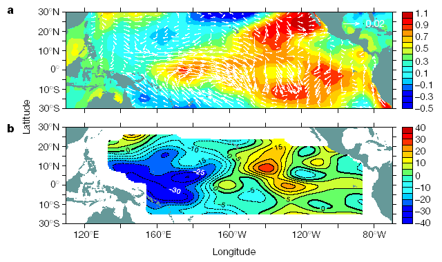
Figure 3. Decadal differences in the tropical Pacific between 1990–99
and 1970–77. a, Wind stress difference (in N m![]() )
for 1990–99 minus 1970–77, based on the Florida State University
wind product (Goldenberg
and O'Brien, 1981). Overplotted is the difference in sea surface temperature
(in °C) the same
time period (Smith et
al., 1994). b, Depth difference (in m) of the 25.0
kg
m
)
for 1990–99 minus 1970–77, based on the Florida State University
wind product (Goldenberg
and O'Brien, 1981). Overplotted is the difference in sea surface temperature
(in °C) the same
time period (Smith et
al., 1994). b, Depth difference (in m) of the 25.0
kg
m![]() potential
density
surface
for 1990–99 minus 1970–77.
potential
density
surface
for 1990–99 minus 1970–77.
