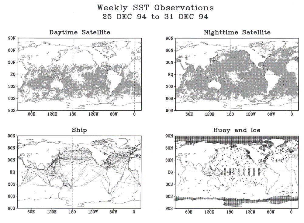
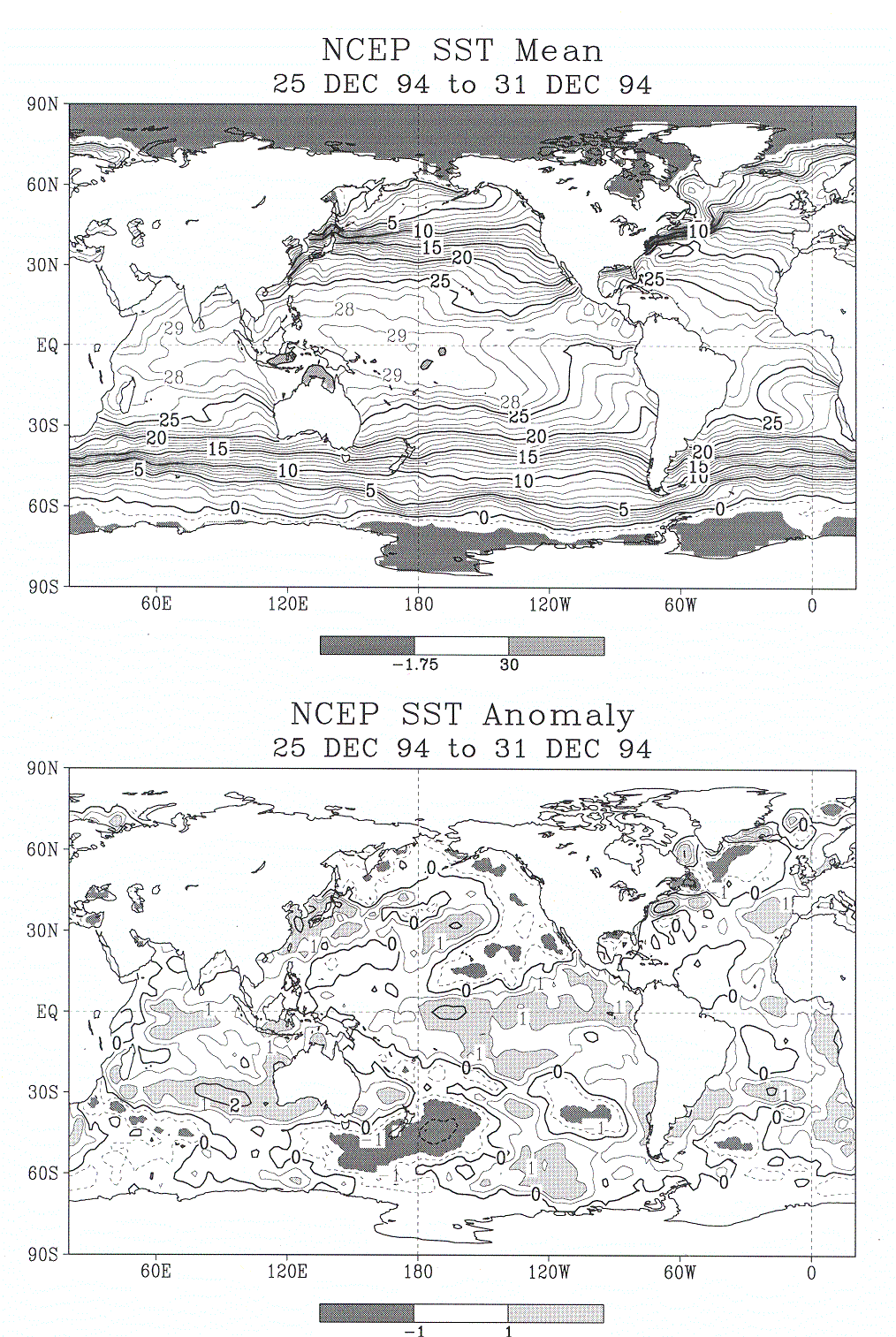
Errors in the 1982 sea surface temperature (SST) analyses discussed in Appendix A led to improved analyses at the NCEP, formerly NMC (Figure C1). These analyses used both in situ and satellite data. The satellite observations are infrared measurements from the AVHRR on the NOAA polar orbiting satellites. These data were processes operationally by NOAA's Environmental Satellite, Data, and Information Service (NESDIS) until 1993, when the responbility for operational processing was transferred to the Naval Oceanographic Office of the U.S. Navy [May et al., 1998]. The satellite SST retrieval algorithms are "tuned" by regression against quality-controlled drifting buoy data using the multichannel SST technique of McClain et al. [1985] and Walton [1988]. This procedure converts the satellite measurement of the "skin" SST (roughly a millimeter in depth) to a buoy "bulk" SST (roughly at 0.5 m depth). The tuning is done when a new satellite becomes operational or when verification with the buoy data shows increasing errors. The algorithms are computed globally and are not a function of position or time. Although the AVHRR cannot retrieve SSTs in cloud-covered regions, the spatial coverage of satellite data is much more uniform than the coverage for in situ data. As an example, the distribution of AVHRR retrievals for the last week of TOGA is shown in Figure C1, where the number of daytime and nighttime observations has been averaged onto a 1° spatial grid. Day and night have been separated because the cloud detection algorithms are different for day and night.
Figure C1: Number of SST observations for the week of December 25–31. (top) Regions on a 1° grid where the number of daytime or nighttime AVHRR retrievals is three or more. (bottom) The distribution of ship, buoy, and simulated ice SSTs. In Figure C1 (bottom right) the moored buoys are indicated by a circle, the drifting buoys by a dot, and the ice by a plus.
In situ SST data used in the NCEP analyses are obtained from two different sources. The data source from 1990 to present consists of all ship and buoy observations available to NCEP on the GTS within 10 hours of observation time. Prior to 1990, the data were obtained from the COADS [Woodruff et al., 1987]. COADS adds additional delayed data to the GTS data. After a wait of several years the procedure can roughly double the number of in situ observations. The distribution of real-time in situ data for the last week of TOGA is shown in Figure C1. Figure C1 (top) shows the distribution of observations from ships. These observations are surface marine observations, which are roughly 20 times more frequent than XBT observations. This distribution depends on ship traffic and is most dense in the midlatitude northern hemisphere. Figure C1 (bottom) shows the in situ observations from drifting and moored buoys. The deployment of the buoys has partially been designed to fill in some areas with little ship data. This process has been most successful in the tropical Pacific and southern hemisphere. However, it should be noted that there are areas, such as the tropical Atlantic, that have almost no buoy SST observations.
In situ and satellite observations are sparse near the ice edge. To supplement these data, sea ice information is used on a 2° grid. If a grid box is ice covered (concentration of 50% or greater), an SST value is generated with a value of -1.8°C, which is the freezing point of seawater with a salinity of 33–34 psu. This range of salinity is typical near the ice edge in the open ocean.
The superior coverage and greater density of satellite SST data would tend to overwhelm the in situ data in most conventional analyses. This would only be a problem if the satellite data have biases on large timescales and space scales. These biases have occurred in the operational satellite data set. The most severe cases occurred following the March–April 1982 eruptions of El Chichon [Reynolds et al., 1989b] and the June 1991 eruptions of Mount Pinatubo [Reynolds, 1993]. The stratospheric aerosols from these eruptions resulted in strong negative biases in the satellite algorithms.
To illustrate the effect of one of these events, the average weekly anomaly from in situ, daytime, and nighttime satellite observations was computed between 20°S and 20°N during the period with strong stratospheric aerosols from Mount Pinatubo [see Reynolds, 1993]. The results (Figure C2) show that the SST anomalies were all tightly grouped during May and June 1991. After this period the in situ anomaly remained relatively constant while the day and night satellite anomalies became more negative. The nighttime anomalies reached a minimum during September; the daytime retrievals reached a minimum during August. The difference between the in situ and satellite anomalies shows that the satellite observations had average negative biases with magnitudes > 1°C in the tropics in August and September 1991. An attempt was made on October 3, 1991, to correct the nighttime algorithm. However, as shown in Figure C2, this correction was only partially effective. As discussed by Reynolds [1993], this correction led to other satellite biases in the southern hemisphere midlatitudes. The aerosols and the associated tropical biases gradually became weaker until the biases became negligible in April 1992.
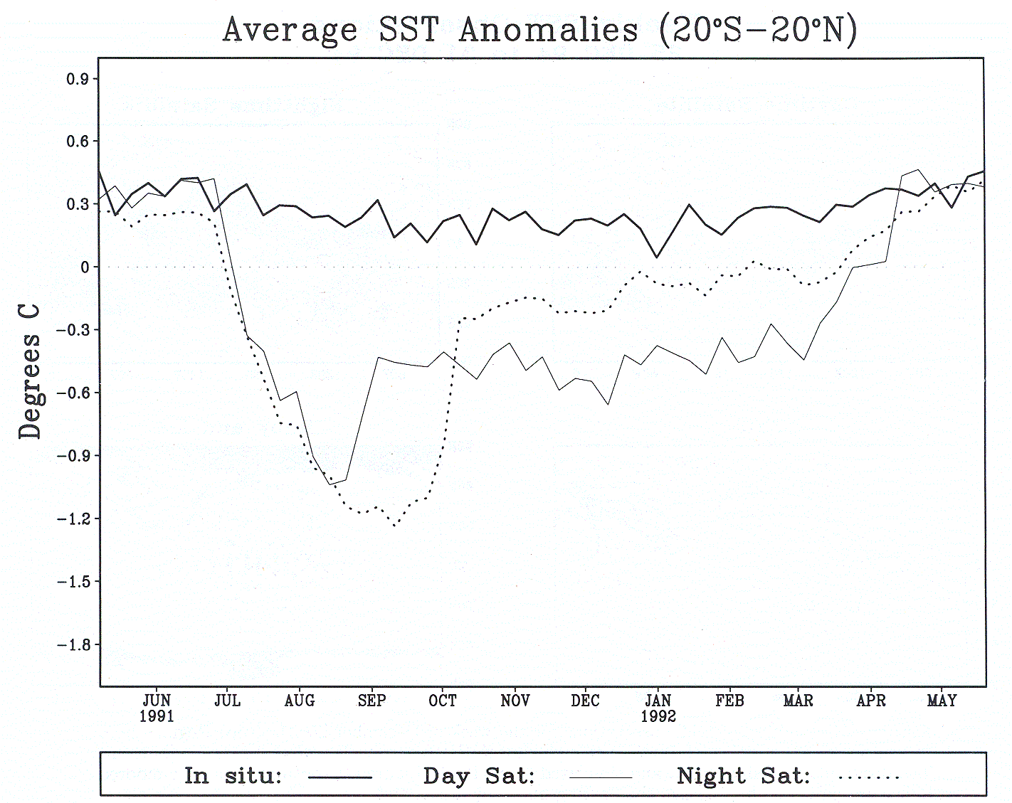
Figure C2: SST anomalies obtained from weekly in situ, daytime, and nighttime satellite observations. The anomalies are averaged between 20°S and 20°N from May 1981 to May 1992 [from Reynolds, 1993].
The NCEP analysis of Reynolds [1988] and Reynolds and Marsico [1993] used Poisson's equation to remove any satellite biases relative to the in situ data before combining the two types of data. This analysis, henceforth called the blend, was produced monthly from January 1982 to December 1994 on a 2° grid with an effective spatial resolution of 6°. In this procedure the analysis resolution was degraded to a resolution that could be supported by the in situ data.
To improve this resolution, an optimum interpolation (OI) analysis was developed [Reynolds and Smith, 1994]. The OI is done weekly on a 1° grid and uses the same data that were used by the blend. To correct for satellite biases, a preliminary step using the blended method provides a smooth correction with 12° resolution for each week. The satellite data are adjusted by this correction and used in the OI along with the in situ data. In the next step, OI error statistics are assigned to each type of data (ship, buoy, etc.). The random in situ and satellite data errors are comparable. Hence, because the satellite distribution is so much better than the in situ distribution, the satellite data overwhelm the in situ data in the OI. The OI also weights the nighttime temperatures more since the diurnal cycle is not fully resolved and the daytime temperatures tend to be noisier.
The OI has now been computed from November 1981 to the present. As an example, the analysis corresponding to the data coverages shown in Figure C1 was presented earlier in Figure 4. November 1981 was selected as the starting point of the OI analysis because that is the date the AVHRR data first became operational. For comparison the OI has also been computed without the preliminary satellite bias correction. This analysis will be referred to as OI-UC, where UC stands for uncorrected.
To verify the accuracy of the differences among the blend and the two versions of the OI, monthly SST anomalies from the analyses are compared with independent data. These data are the monthly averaged SST anomalies from TOGA-TAO equatorial current moorings [McPhaden, 1993a]. Three locations have been selected with the longest records: 110°W, 140°W, and 165°E. The monthly root-mean-square (rms) difference between buoys and each of the three analyses (blend, OI, and OI-UC) are computed for the period January 1982 to January 1993 and for each month. The results are summarized in Table C1 for a high aerosol year, 1991, and for the entire period. In all cases the OI is superior to both the OI-UC and the blend. The OI is superior to the blend because of its better resolution. The spatial gradients are greater in the eastern than in the western Pacific, so analysis differences between the blend and the OI are greater at 110°W and 140°W than at 165°E. In years without strong satellite biases the OI and OI-UC analyses behave similarly. However, the large biases during periods such as 1991 cause the degradation of OI-UC analysis relative to both the OI and the blend.
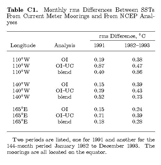
Table C1. Monthly rms Differences Between SSTs From Current Meter Moorings and From NCEP Analyses
The OI analysis with the satellite bias correction yields high-quality global SST fields. These SST fields are widely used for climate monitoring, prediction, and research as well as specifying the surface boundary condition for numerical weather prediction. They appear in many publications, e.g., the NCEP Climate Prediction Center's Climate Diagnostic Bulletin, and are freely available to any user. The SST fields have also been used in atmospheric reanalyses at NCEP, ECMWF, and the U.S. Navy.
In addition, the OI fields have also been used to improve SST analyses from 1950 to 1981 when satellite data were not available. In this method, spatial patterns from empirical orthogonal functions (EOFs) are obtained from the OI fields. The dominant EOF modes (which correspond to the largest variance) are used as basis functions and are fit in a least squares sense to the in situ data to determine the time dependence of each mode. A complete field of SST is then reconstructed from these spatial and temporal modes as described by Smith et al. [1996].
At the beginning of the TOGA project in 1985 it seemed unlikely that satellite altimetry would play much of a role in the ocean observing system. No altimeters had flown since Seasat 7 years earlier. The proposed Seasat-like Navy Remote Ocean Sensing System (NROSS) collapsed under the weight of its enormous budget. NASA had struggled for years, without success, to obtain approval for its dedicated ocean topography altimeter TOPEX, and the French were having similar problems with their counterpart, known as POSEIDON. The U.S. Navy was preparing for the launch of Geosat in March 1985, but this was to be a classified geodetic mission, and it was doubtful that any of the data would be available to the scientific community. On a positive note the European Space Agency (ESA) had just begun building ERS-1 with its altimeter, but the mission was several years behind its original 1987 launch schedule. Given this background, it is easy to understand why TOGA planned to rely so heavily on in situ observations rather than remote sensing.
Despite these inauspicious beginnings, satellite altimetry ultimately provided global observations during 8 of the 10 TOGA years, the gap occurring during 1989–1991 between Geosat and ERS-1. Some of the Geosat data were initially classified, but today they are available in their entirety, spanning the first 4 years of the TOGA project. The Geosat era turned out to be one of the more interesting times in the tropical Pacific cycle because it included a normal period (1985 through mid-1986) followed by distinct ENSO warm and cold events in 1986–1987 and 1988–1989, respectively. ERS-1 became operational in 1991 just as another warm event was beginning, and the TOPEX/POSEIDON observations began in 1992. With the successful launch of ERS-2 in 1995, three altimeters were collecting data simultaneously by middecade, with excellent prospects for a continuous series of altimeters to be in place for the foreseeable future. As shown in Figure C3, it has been possible to connect the various altimeter missions to generate a consistent, long-term record of sea level variations throughout the tropics.
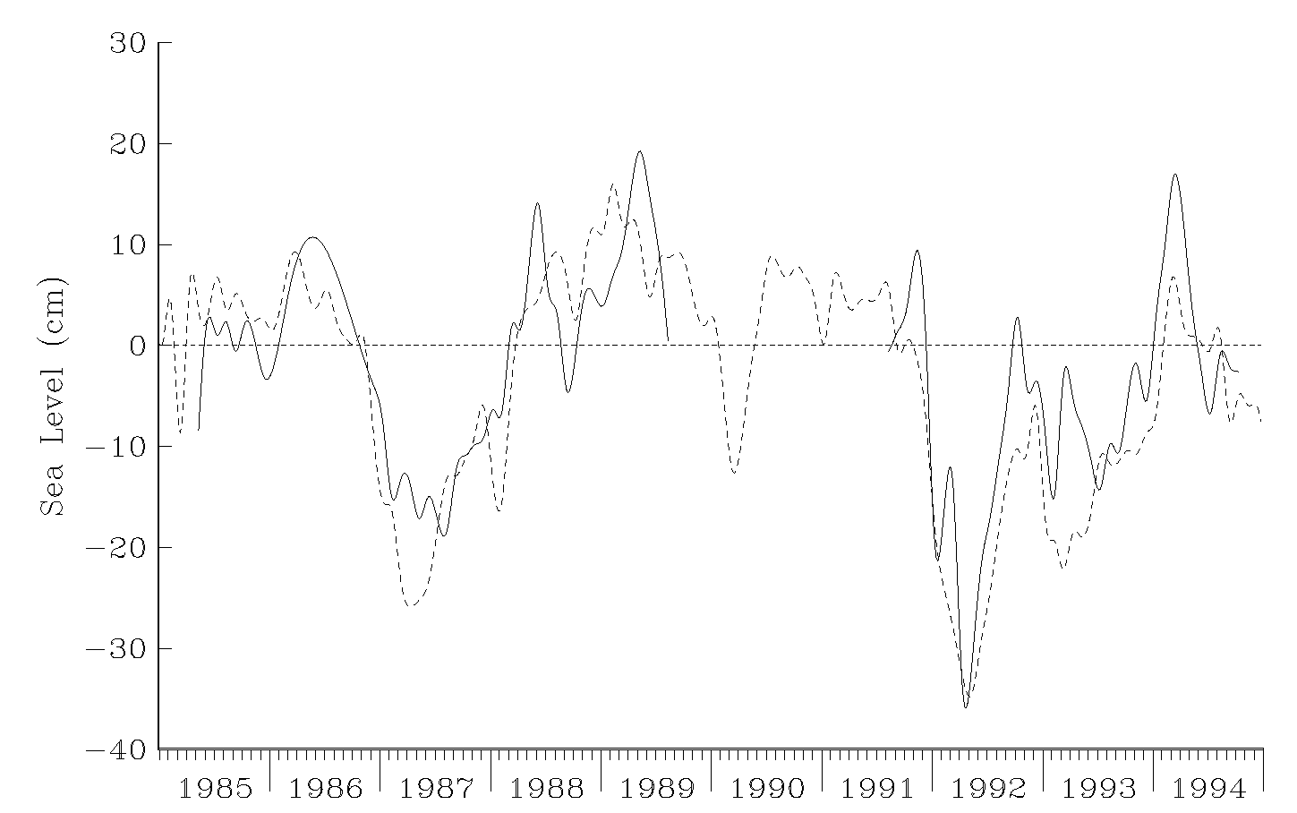
Figure C3: Sea level time series computed from Geosat, ERS-1, and TOPEX/POSEIDON altimeter data (solid line) near the Honiara tide gauge (dashed line) in the western tropical Pacific (taken from Lillibridge et al. [1994]).
The spatial and temporal sampling patterns have varied among these missions as summarized by Koblinsky et al. [1992], but of more fundamental importance is their relative accuracies. It is useful to begin with TOPEX/POSEIDON, as this highly accurate altimeter system has set the standard by which all others are being measured. Primarily because of advances in orbit determination, TOPEX/POSEIDON is able to measure sea level with an absolute accuracy of 4 cm for 1-s averages [Fu et al., 1994; Tapley et al., 1996]. For monthly means in 2° squares the figure is closer to 2 cm [Cheney et al., 1994], and global sea level is being monitored at the level of a few millimeters [Nerem et al., 1997]. Geosat and ERS-1, even after recent orbit improvements [Scharoo et al., 1994; Williamson and Nerem, 1994] are only accurate to 10–15 cm in an absolute sense for the 1-s data. But simple adjustments [Lillibridge et al., 1994] and other sophisticated processing techniques [Tai and Kuhn, 1995] have increased the net accuracy to 5 cm or less for determination of monthly mean sea level variations. Furthermore, much of the ERS-1 error can be removed by adjusting the profiles relative to concurrent TOPEX/POSEIDON data [Le Traon et al., 1995]. For most tropical ocean applications the result is a nearly continuous altimetric record of sea level variability, which can be assimilated in ocean models to improve initial conditions for climate forecasting [Fu and Cheney, 1995].
Special altimeter validation efforts were undertaken during TOGA in recognition of the fact that accuracy requirements might be higher for sea level near the equator than elsewhere in the world ocean. The primary goal of satellite altimetry missions is the study of large-scale ocean circulation, through estimation of the surface geostrophic currents. Geostrophic estimates of surface flow will be very sensitive to small sea level errors near the equator, however, because of the vanishing of the horizontal component of the Coriolis force [e.g., Picaut et al., 1989]. A rigorous open-ocean validation experiment was therefore conducted in the western equatorial Pacific Ocean during the verification phase of the TOPEX/POSEIDON mission to examine the accuracy of the altimetry measurements in the TOGA domain. Two TAO moorings were outfitted with additional temperature, salinity, and pressure sensors to measure within 1 cm the dynamic height from the surface to the bottom at 5-min intervals directly beneath two TOPEX/POSEIDON crossovers; bottom pressure sensors and inverted echo sounders were deployed as well [Katz et al., 1995a; Picaut et al., 1995]. Instantaneous comparisons with the 1-s TOPEX/POSEIDON altimeter retrievals and the 5-min dynamic height resulted in a root-mean-square difference as low as 3.3 cm at 2°S–164°E and 3.7 cm at 2°S–156°E. After the use of a 30-day low-pass filter, in situ and satellite data were found to be highly correlated, with rms differences of < 2 cm.
The applicability of satellite altimeter data for estimating zonal surface current variability at the equator was also assessed using the meridionally differenced form of the geostrophic momentum balance [Picaut et al., 1990; Delcroix et al., 1991, 1992; Menkes et al., 1995]. These studies indicated that altimetry-derived geostrophic zonal current estimates agreed well with near-surface zonal currents observed from TAO moorings along the equator. Given the sensitivity of the geostrophic approximation to small sea level variations near the equator, these results represent the most stringent test of using altimetry observations to estimate sea level and surface currents anywhere in the world ocean.
For several years before the beginning of TOGA, there was optimism that the 1978 success of Seasat, which, for the first time, recorded surface wind velocity over the global ocean [Chelton et al., 1989], would be followed by another satellite wind velocity measuring system. In 1986, cancellation of the NROSS mission, which was to have carried a NSCAT to measure surface wind velocity, created a requirement to implement an in situ surface wind velocity measurement system throughout the equatorial Pacific. This requirement was in part met by development of the TOGA-TAO array [Hayes et al., 1991a; McPhaden, 1993a] using moored wind measurement technology developed in earlier Pacific climate studies [Halpern, 1988b].
The inability during TOGA to launch NSCAT, which was intended to provide global coverage of 25-km-resolution surface wind velocity every 3 days, was partially mitigated with the July 1991 launch of ERS-1. Monthly mean ERS-1 wind speed and direction are accurate to about 1 m s-1 and 35°. However, at wind speeds below 2–3 m s-1, accuracy is poor because the intensity of Bragg scattering has little variation with wind speed. However, ERS-1 data yielded the first opportunity to learn about the detailed space-time structures of intraseasonal surface westerly wind bursts along the Pacific equator [Liu et al., 1996].
In the interim from the beginning of TOGA to the launch of ERS-1, special sensor microwave imager (SSM/I) surface wind speed measurements, which have been recorded since July 1987, have been combined with wind directions [Atlas et al., 1991]. The Atlas et al. [1991] SSM/I surface wind velocity data product, which Busalacchi et al. [1993] demonstrated to be an alternate source of wind vector information, yielded sea surface temperatures, simulated from an ocean general circulation model, that were more representative than those created with a numerical weather prediction surface wind data product [Liu et al., 1996].
The ERS-1 scatterometer and the SSM/I represent active and passive microwave wind-measuring tech- niques, respectively. Another active microwave method is produced with the radar altimeter, which is of secondary importance for studies of large-scale ocean circulation because of the very small coverage in the cross-track direction. SSM/I and ERS-1 wind data are determined over distances > 500 km perpendicular to the ground track, with an areal coverage nearly 100 times greater than that of an altimeter.
Return to Appendix B or go to Appendix D