U.S. Dept. of Commerce / NOAA / OAR / PMEL / Publications
We have shown that the commonly observed intraseasonal Kelvin waves in the equatorial Pacific are generated by the fluctuations of winds and tropical convection associated with the MJO. In particular, the waves exhibit low-frequency modulation due to annual and interannual variations of west Pacific convection, which itself is a signal propagating from further west. Since the MJO life cycle is sensitive to the distribution of warmest SST over both the Indian and Pacific Oceans, and to the planetary atmospheric circulation, the oceanic signal must be taken to be a manifestation of a global phenomenon, and not simply internal to the Pacific. Although it is easy to see how low-frequency variations of SST in the Pacific can affect the MJO, which has its intense convection signals over the warmest SST, we now ask whether the MJO events themselves could have a role in the interannual variations of the Pacific. Such a process would require a nonlinear coupling between the relatively high intraseasonal frequencies and a rectified low-frequency response.
One mechanism that might produce this interaction is suggested by the 500- to 1000-km intraseasonal bumps on the SST contours in Figure 5, which occur both in the eastern and western Pacific. SST variability at this timescale, in the absence of corresponding atmospheric forcing, points to zonal advection by the intraseasonal Kelvin waves as a possible explanation. In view of the fact that convection and westerly winds follow the warmest water eastward, this could provide a mechanism by which intraseasonal variability in the ocean can feed back to affect the atmosphere. Since the atmosphere can respond to SST forcing (by shifting the location of convection) much more rapidly than the ocean responds to changing winds, each eastward advection event can draw subsequent convection further east.
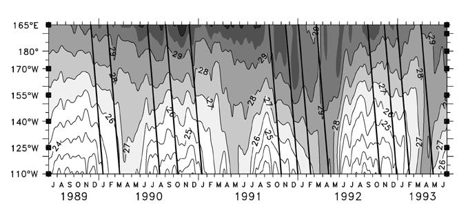
An apparent example of this process occurred during the basin-wide warming
of the El Ni±o of 1991-1992. Figure 12a shows
a detail of the SST zonal section from Figure 5
for the period July 1991 through April 1992. Overlaid on the SST contours and
shading are, first, the zero contour of the zonal winds (same data as Figure
4) showing the advance-and-retreat eastward expansion of westerlies, and
second, the Kelvin wave propagation lines from Figure
3 showing the four downwelling waves (associated with eastward current anomalies)
observed in 20░C depth during the onset of the 1991-1992 warm event. The second
and third westerly events, in November 1991 and January 1992, each extended
about
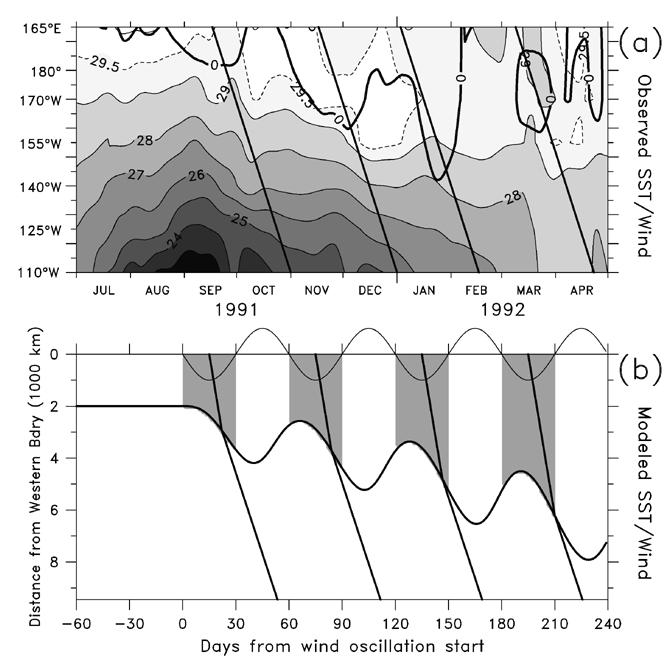
Figure 12. (a) Detail of SST on the equator for July 1991 through April 1992 (during the peak of the El Ni±o of 1991-1992). Contours and shading show SST with a contour interval of 1░C, with supplemental contour/shade at 29.5░C. Light contours show warmer temperatures (opposite of Figure 5). The heavy slant lines are the same Kelvin lines shown in Figure 3. The heavy contour labeled "0" is the zero line of zonal winds, showing the steplike progression of westerlies eastward over the Pacific during the onset of the warm event. (b) Model SST/wind to match the timing of Figure 12a. Output of the simple model described in section 4. The heavy curve is the eastern edge of the 29░C SST and the wind patch (the result of integrating (3); see text). The light sinusoidal curve at top is the time series of winds from (1) (up is easterly, down is westerly) (winds are zero before day 0). The shading shows the region of westerly winds. Slant lines indicate maximum positive pressure perturbation to match the observed Kelvin lines in Figure 12a; east of the forced region these are Kelvin characteristics, within the forced region they move at speed 2c (see text).
Kessler and McPhaden [1995b] studied the zonal advective effect on SST at 140░W during the 1991-1993 El Ni±o and showed that although this forcing was not the most important term in the SST balance at annual and interannual frequencies it was dominant during the period of intense intraseasonal variability at the height of the warm event. Figure 13 compares the advective terms d(SST)/dt and ud(SST)/dx at 0░, 140░W (d(SST)/dx is estimated by centered difference between 155░W and 125░W) during the same period as Figure 12a for SST and winds. The positive (warming) humps of -ud(SST)/dx in Figure 13 show the advection due to the intraseasonal Kelvin waves at 140░W in October and November-December 1991 and January 1992. Clearly, the first major warming that took place in September was not the result of Kelvin advection, but the next two events are quite consistent with that interpretation, and the two terms balance closely. The final warming in March occurred before the passage of the fourth Kelvin wave and again was apparently not due to that wave. The fourth wave produced only a very weak advective signal in Figure 13 because the zonal temperature gradient at 140░W was near zero at that time (Figure 12a).
The net result of successive intraseasonal waves associated with steplike eastward
movement of the warmest water and westerly winds appears as a much lower-frequency
signal. In this view, Figure 12a suggests that
zonal advection moved the 29.5░C water
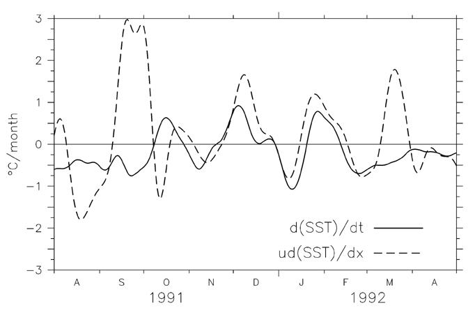
Figure 13. Comparison of d(SST)/dt and ud(SST)/dx at 0░, 140░W. The solid line shows -ud(SST)/dx, where u is taken as the 14-m (shallowest level) zonal current measured by ADCP and d(SST)/dx is estimated by centered difference between 125░W and 155░W. The dashed line is d(SST)/dt at 140░W. Both time series are filtered with a 17-day triangle filter. Upward on the plot indicates a warming tendency for both time series.
A simple coupled model illustrates the dynamics involved. The model is not intended to be a realistic simulation of all or even most aspects of the onset of El Ni±o, but simply to show that a nonlinear interaction between the oceanic intraseasonal Kelvin waves and the Madden-Julian Oscillation is possible. The model is highly idealized to represent the single mechanism of an advective feedback between intraseasonal advection of SST and the rapid response of the atmosphere to changes of location of the warm pool. This feedback may be an element of the slow eastward advance of warm SST and atmospheric convection that has been noted to occur during the onset of warm events.
Assume that the initial state of the ocean has a warm pool extending eastward from the western boundary. Let sinusoidally oscillating, zero-mean zonal winds occur only to the west of a particular value of SST, say the 29░C isotherm. The frequency and phase of the surface winds is assumed to be fixed by upper atmosphere waves oscillating at a Madden-Julian timescale, but their longitudinal extent is determined by the SST. For simplicity, we assume that the winds do not vary in longitude within the wind patch (from the western boundary to the 29░C SST isotherm), but are zero outside the patch. In the ocean, Kelvin waves forced by the oscillating winds advect the 29░C patch edge. We assume a simple ocean dynamics such that the ocean response to winds is that the forced ocean current is directly proportional to the wind integrated over the Kelvin wave characteristic. Other than zonal advection, due to Kelvin wave passage or to wind forcing directly, there are no processes that affect SST in this model.
This model can be formulated as follows. The western boundary is at x = 0. Let x = a(t) mark the (time varying) east edge of the 29░C SST/wind patch. Then the wind field is
![]() (1)
(1)
where b is the (constant) amplitude of the wind and  the frequency. Note that uatmos has zero mean. The ocean current
at the patch edge is now taken to be directly proportional to the wind integrated
over the patch along the Kelvin wave characteristic. The integral sums the forcing
felt by a wave since it left the western boundary.
the frequency. Note that uatmos has zero mean. The ocean current
at the patch edge is now taken to be directly proportional to the wind integrated
over the patch along the Kelvin wave characteristic. The integral sums the forcing
felt by a wave since it left the western boundary.
 (2)
(2)
where b* is the (constant) coupling efficiency, c
is the Kelvin wave speed, and ta is the arrival time of Kelvin
characteristics at the patch edge. The coupling efficiency b*
scales the speed of the current generated by a given wind, and is a tunable
parameter in this model. For simplicity of notation, we combine bb*
= B, which has units of (time)-1 and incorporates the effects
of both wind strength and coupling efficiency; thus B represents the
net forcing amplitude felt by the ocean. Since the wind does not vary (in x)
for 0  x
a(t), the integration can be performed in time alone from t
= ta - a/c (the time a characteristic leaves
x = 0) to t = ta, as indicated in (2). Since
the patch edge position a(t) is changed only by zonal advection,
we identify uocean = da/dt = rate of change
of position of the patch edge. Carrying out the integral in (2),
x
a(t), the integration can be performed in time alone from t
= ta - a/c (the time a characteristic leaves
x = 0) to t = ta, as indicated in (2). Since
the patch edge position a(t) is changed only by zonal advection,
we identify uocean = da/dt = rate of change
of position of the patch edge. Carrying out the integral in (2),
 (3)
(3)
This is a nonlinear (because a(t) appears in the argument to
the cosine on the right-hand side) ordinary differential equation, which can
be easily integrated numerically. We see from (3) that da/dt is
zero for a = 0 (no patch) or for a = 2 c/
(a patch with width the same as the wavelength of a Kelvin wave of frequency
c/
(a patch with width the same as the wavelength of a Kelvin wave of frequency
![]() ), so these are limiting
equilibrium positions where the motion stops, but the motion can be of either
sign between these two locations.
), so these are limiting
equilibrium positions where the motion stops, but the motion can be of either
sign between these two locations.
Reasonable values of the model parameters can be chosen as follows. We have
established that the Kelvin wave speed is c =
= 2![]() /(60 days). The wind
forcing amplitude B can be estimated from the wind-forced linear zonal
momentum equation
/(60 days). The wind
forcing amplitude B can be estimated from the wind-forced linear zonal
momentum equation
![]() (4)
(4)
where  =
=  acDua2
(subscripts a and o here indicate atmosphere and ocean, respectively,
and cD is the drag coefficient), and H is the thickness
of the wind-forced layer. Taking usual values a
= o
=
acDua2
(subscripts a and o here indicate atmosphere and ocean, respectively,
and cD is the drag coefficient), and H is the thickness
of the wind-forced layer. Taking usual values a
= o
= 
Note that the estimate of the tunable parameter B from (4) is proportional
to the wind speed squared and also that the choice of the wind-driven layer
depth is somewhat arbitrary. In any case, the model has a simple parameter space,
and the response is qualitatively the same for all values  .c/
(and note that the equilibrium value is not a function of the wind forcing parameter
B, but only of the unambiguous quantities c and ).
For (unrealistically) large values of B the solution can jump to an integer
multiple of 2c/
but then resumes identical behavior approaching the new equilibrium position.
The model is also not sensitive to the starting phase of the wind. In the example
discussed in section 4.3 and shown in Figure 12b
we have started the winds at the beginning of their westerly phase at time zero
(winds are zero before t = 0), but if the winds are started easterly
at t = 0, the process takes several more oscillations before rapid growth
occurs, but the eventual result is the same.
.c/
(and note that the equilibrium value is not a function of the wind forcing parameter
B, but only of the unambiguous quantities c and ).
For (unrealistically) large values of B the solution can jump to an integer
multiple of 2c/
but then resumes identical behavior approaching the new equilibrium position.
The model is also not sensitive to the starting phase of the wind. In the example
discussed in section 4.3 and shown in Figure 12b
we have started the winds at the beginning of their westerly phase at time zero
(winds are zero before t = 0), but if the winds are started easterly
at t = 0, the process takes several more oscillations before rapid growth
occurs, but the eventual result is the same.
The behavior of the solution is shown in Figure
12b. The patch edge moves east in pulses not dissimilar to those observed
(Figure 12a) for SST and westerly winds during
late 1991. Each step advances about 1000-c/
(in the present example 2c/
=
The solution has a basic similarity to the results of a coupled general circulation model simulation reported by Latif et al. [1988]. They added a single 30-day westerly wind event to their model after spin up with annual cycle forcing and then let the coupled system run freely. The model responded with an initial rapid eastward shift of the SST maximum toward the central Pacific due to zonal Kelvin wave advection, then subsequently the model atmosphere developed persistent westerlies blowing toward the warmest water. This kept the central basin sea level and SST high for at least a full year after the single 30-day imposed forcing event. Although the Latif et al. [1988] model is much more complex than the present formulation, it appears that the coupled dynamics are similar in this case, with the atmosphere responding to transient eastward displacement of warm SST by developing westerlies that serve to maintain and extend the SST pattern.
The key dynamics that produce the rectified low-frequency outcome from the high-frequency forcing is that the model atmosphere responds immediately to the state of the SST, while the ocean's response to the atmosphere is lagged because it is due to an integration over forcing of finite duration. While the model is crude, this timescale difference between the two fluids is probably representative of a true distinction. The other important characteristic of the model formulation is that the strength of the model ocean response is proportional to the fetch, so that westerly winds, which advect the patch edge eastward, increase the fetch, while easterly winds reduce it. Thus during westerly periods the increasing fetch means the response increases, but during easterly periods the decreasing fetch produces a weaker signal, so each westward retreat is somewhat weaker than the eastward advances. This behavior is much like the observations in late 1991.
We noted in the introduction that the Madden-Julian Oscillation is a global phenomenon, but its surface expression is strong only over the warm-SST part of the equatorial ocean. Similarly in the model, we assume that the forces that establish the basic oscillation are entirely external to the feedback mechanism. In this representation the atmospheric dynamics of the MJO set the 60-day oscillation period, while the SST determines only the zonal length of the region in which convection and strong low-level winds develop during the phase favorable to upper-level divergence. Although the existence of the MJO probably requires a minimum size warm SST region to exist, the few-thousand-kilometer changes during a single event may be small perturbations to the global state SST felt by the atmosphere, and thus the interaction described here may not strongly affect the fundamental dynamics or frequency.
Several important weaknesses of the model are evident. We neglect entirely
any heat exchange between the atmosphere and ocean, which is obviously crucial
to the evolution of the coupled system. The present, highly-idealized formulation
can only be relevant over short time scales during which the rapid advection
that occurs as a result of the intraseasonal waves can be the dominant process
affecting SST. Such dominance of intraseasonal Kelvin wave-mediated zonal advection
on SST change can occur during warm event onset and was observed at 140░W during
November 1991 through February 1992 (section 4.1 and Figure
13). Second, the model implicitly has an infinite heat reservoir that allows
the warm pool to expand indefinitely, determined only by dynamics, not a heat
balance. However, the same result would still occur if eastward advection in
the warm pool exposed cooler water to the west, if one makes the reasonable
assumption that the convection and westerlies advance over the cool water to
the warm pool. Similarly, SST cooling due to evaporation associated with the
increase in absolute wind speeds during westerly events in the western Pacific
is typically less than 1░C, which is not enough to reduce the absolute temperature
to below the threshold needed for deep convection. Therefore the primary feedback
shown by the simple dynamics would not change if the model was made more realistic
by allowing changing SST under the winds. However, such cooling may well have
been the reason for the slight decrease in warm pool SST under the strong winds
of January 1992 (Figure 12a). Third, in order
to demonstrate without ambiguity that the slow change in the ocean can be due
entirely to the coupled feedback rectification, we have postulated zero mean
wind forcing. In the real event, it is observed that the onset of El Ni±o occurs
in a regime of low-frequency westerly forcing with the higher-frequency convection
events superimposed (Figure 3, top). This would
tend to make the eastward advective signal stronger, but the aim here is to
show that it is not necessary to have mean westerly forcing in order to get
a net eastward propagation in the ocean. Fourth, to achieve maximum mathematical
simplicity, we have specified that the winds do not vary in x within
the wind patch (equation (1)). In fact, the wind signal propagates eastward
with the convection signal at speeds of the order of
An element of the ocean dynamics that we have ignored is the Rossby waves that
would also be generated by the oscillating forcing. Rossby waves might affect
the result in three ways. First, the Kelvin waves discussed here would produce
Rossby waves upon reflection at the eastern boundary. However, a variety of
studies [du
Penhoat et al., 1992; Kessler
and McCreary, 1993; Kessler
and McPhaden, 1995a; Minobe and Takeuchi (Annual period equatorial waves
in the Pacific Ocean, submitted to Journal of Geophysical Research, 1994))
have suggested that these waves will not survive propagation across the entire
Pacific, thus we think this would not be a major element of a more complete
solution. Second, the oscillating winds would generate Rossby waves directly.
These waves propagate west, and so would not influence the east edge of the
patch, except by producing secondary Kelvin waves upon reflection from the western
boundary. The amplitude of the Rossby waves forced by the wind patch depends
on the meridional shape of the wind field; the amplitude of the consequent reflected
Kelvin waves depends on the mix of Rossby meridional wavenumbers and the shape
of the western boundary [Clarke,
1983; McCalpin,
1987; Kessler,
1991]. The phase of the resulting Kelvin waves depends on the zonal width
of the patch, and we can anticipate that as the patch length changes the Kelvin
waves due to boundary reflection will exhibit varying phase compared to the
directly forced waves and may be of either sign relative to the original solution.
The time lag for Rossby wave propagation from the patch edge to the western
boundary and then Kelvin wave propagation back to the patch edge a can
be written tR =
A third way in which our neglect of Rossby waves in the model is unrealistic
is that there can also be easterly wind anomalies to the east of the convection
on MJO timescales, and these would generate Rossby waves carrying equatorial
currents westward toward the patch edge that would oppose the Kelvin signals
modeled here. It is not straightforward to model these Rossby waves in the context
of a model as simple as the present one, since the zonal width of the easterly
forcing is much harder to define than the width of the convective region. Also
note that the much slower Rossby propagation speed (1/3 of the Kelvin speed
for first-meridional-mode waves) implies that a reasonably sized easterly patch
region of c/,
and the integral over the characteristic would thus be small (see discussion
of equation (6) and Figure 14 in section 4.6).
In addition, we have noted that the central Pacific intraseasonal zonal wind
variability is very much weaker than that over the warm pool (see Figure
4). In sum, we conclude that our neglect of the Rossby wave forcing, while
unrealistic, does not distort the fundamental feedback properties of the model.
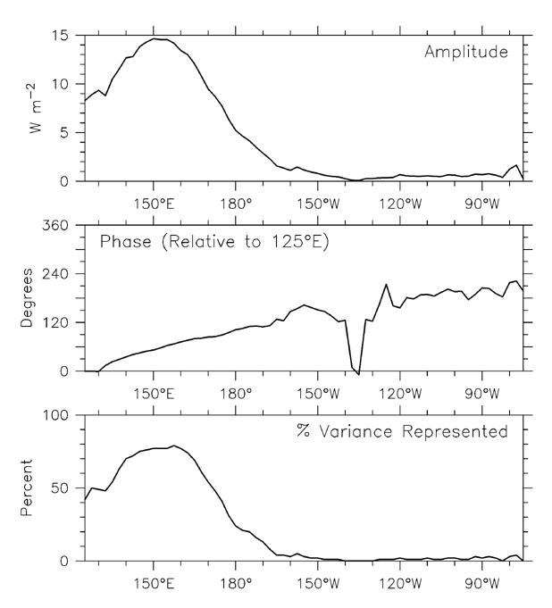
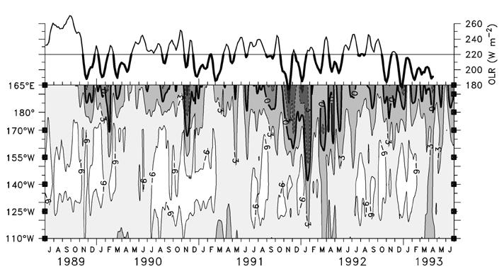
Figure 14. Complex (frequency domain) EOF 1 of intraseasonal (30- to 80-day period) OLR along the equator in the Pacific during 1979-1993. (Top) Amplitude (W m-2) of the complex eigenvector. The zonal structure of this EOF is used to estimate the zonal length of the OLR patch (see text). (Middle) Phase relative to 125░E. The slope in the western Pacific indicates eastward propagation at a speed of about 4.5 m s-1. (Bottom) Percent variance represented.
Recognizing that all these dynamic and thermodynamic weaknesses and crude approximations to the observations make the model unsuitable for realistic simulation of the coupled system in general, the extremely simple form used here was chosen for the purpose of isolating a particular process that may be relevant to the real system during a limited (but perhaps important) period.
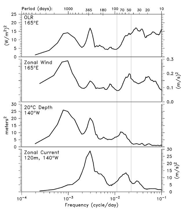
We have shown (in agreement with previous studies) that although intraseasonal
variability in the atmosphere was centered at 35- to 60-day periods (Figure
6), the ocean response was shifted toward the lower-frequency end of the
band. Thermocline depth and undercurrent speed variability were very weak at
periods less than c/).
For the 60-day waves discussed above, this distance is
Using terminology analogous to the model (1)-(3), but with the patch edge fixed (no feedback), let A be the (fixed) east edge of the warm SST/wind patch. The wind field is still described by (1), substituting the constant A for the previously variable a(t). Performing the same integration as in (2), again substituting A for a(t), gives an equation analogous to (3) for the zonal current at the east edge A. Since A is fixed, this expression for u(x = A) may be written as the product of a constant amplitude and a time-varying term.
 (5)
(5)
where the first term on the right-hand side is the (constant) amplitude and the second is the time-varying term. The variance of the Kelvin response at A (and thus everywhere east of A) is the amplitude squared
 (6)
(6)
where the function sinc(x)  [x-1
sin(x)], which equals 1 at x = 0, equals 0 at x =
, and thereafter represents a decaying oscillation
for increasing values of x. In (6) the variance falls to zero as the
period decreases toward the value A/c (the time it takes a Kelvin
wave to cross the patch), because then, in summing the integral over the wind
patch, the easterly and westerly contributions to the ocean forcing cancel.
Therefore the amplitude of the ocean response east of equatorial wind forcing
depends on the product A, and for
some values of these parameters the response can vanish.
[x-1
sin(x)], which equals 1 at x = 0, equals 0 at x =
, and thereafter represents a decaying oscillation
for increasing values of x. In (6) the variance falls to zero as the
period decreases toward the value A/c (the time it takes a Kelvin
wave to cross the patch), because then, in summing the integral over the wind
patch, the easterly and westerly contributions to the ocean forcing cancel.
Therefore the amplitude of the ocean response east of equatorial wind forcing
depends on the product A, and for
some values of these parameters the response can vanish.
An estimate of the zonal length scale of the intraseasonal forcing can be made
using OLR, which spans the entire western Pacific (the buoy observations are
not suitable for this purpose since long records are available only east of
165░E). The 1979-1993 history of equatorial OLR was decomposed in complex empirical
orthogonal functions (CEOFs) in the frequency domain [Wallace
and Dickinson, 1972], using frequencies spanning 30- to 80-day periods
to define the intraseasonal band. Figure 14 shows
the amplitude, phase relative to 125░E and percent variance represented by the
first CEOF, as a function of longitude in the Pacific. In the western Pacific,
the first CEOF expresses 50% or more of the intraseasonal variance, with amplitudes
up to
Figure 15 shows the theoretical variance of
zonal current east of a 5000-km patch as a function of frequency, calculated
according to (6), using the Kelvin wave speed
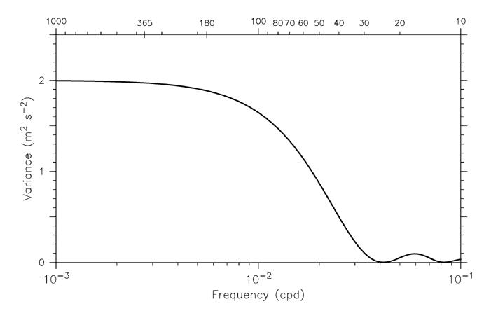
Figure 15. Theoretical variance of zonal current east of a 5000-km width wind patch, calculated according to (6), shown as a function of forcing frequency. The top axis numbering shows the periods in days. Note the rapid drop in variance between 100-day and 30-day periods.
Return to previous section or go to next section