U.S. Dept. of Commerce / NOAA / OAR / PMEL / Publications
The widespread and systematic influence of ENSO on the ocean-atmosphere system
led to the initiation of the Tropical Ocean-Global Atmosphere (TOGA) program,
a 10-year study of climate variability on seasonal to interannual timescales.
One component of the TOGA observing system is the Tropical Atmosphere Ocean
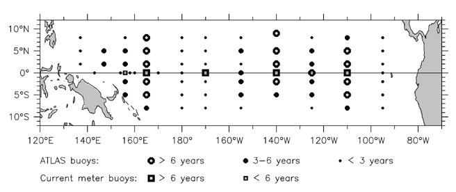
(TAO) buoy array, which consists of more than 60 deep ocean moorings arranged
in ranks nominally 15° longitude apart across the equatorial Pacific (Figure
1). Observations from these moorings form the principal data set used in
this paper. Most of the TOGA-TAO buoys are ATLAS thermistor chain moorings [Hayes
et al., 1991b] that measure temperature at the surface and 10 subsurface
depths down to 500 m, as well as surface winds, relative humidity, and air temperature.
Air temperatures, relative humidities, and water temperatures are sampled 6
times per hour, and daily averages of these are transmitted in real time each
day to shore by satellite via Service Argos. Vector winds
Figure 1. The TOGA-TAO buoy array as of September 1993, showing the approximate length of time the various buoys have been in the water. The present study uses principally the long-term thermistor chain buoys and the current meter buoys, which have been operating for 5 years or longer.
The most important advantage of the buoy data over shipboard observational
techniques is that their high temporal resolution means that intraseasonal frequencies
are not aliased by the ubiquitous high-frequency variability in the ocean [e.g.,
Hayes, 1982; Hayes
and McPhaden, 1992]. However, due to vandalism and instrument failures
of various types, the buoy time series are rarely complete, and some method
for dealing with data gaps is necessary. The history of instrumentation at the
0°, 140°W mooring is shown in Figure 2, indicating
that the time series at most depths are quite gappy and that the mix of samples
changed many times during the decade that a buoy has been in the water at this
location. These changes influence the choice of variables available for study.
For example, although dynamic height might be most useful for some purposes,
there are many periods during which there are no data below
For gaps that are short compared to the period of the signal of interest, it is possible to trade time resolution for gap filling. Chelton and Davis [1982, Appendix] show how to objectively estimate the value of a running mean in the presence of gaps. Their method has been used to fill small (up to about 10 days) gaps by producing a data series filtered with a 17-day triangle (two successive 9-day running means) filter. This filter has a half-power point at 20.3 days and so fills short gaps while retaining the intraseasonal signals of interest here.
The ability to low-pass filter in the presence of gaps also makes possible
the use of complex demodulation on the gappy buoy time series. Complex demodulation
[Bloomfield,
1976] is a type of band-pass filter that gives the time variation of the
amplitude and phase of a time series in a specified frequency band. It may be
preferable to ordinary Fourier techniques when studying a short or gappy record
since the result is local in the sense of being determined only by the data
in the neighborhood of each particular time realization. Briefly, in complex
demodulation the time series is first frequency-shifted by multiplication with
e-i ![]() t,
where
t,
where ![]() is the central
frequency of interest. Then the shifted time series is low-pass filtered (using
the Chelton
and Davis [1982] method if there are gaps), which removes frequencies
not near the central frequency. This low pass acts as a band-pass filter when
the time series is reconstructed (unshifted). The resulting complex time series
can then be expressed as a time-varying amplitude and phase of the variability
in a band near the central frequency; that is, in the form
is the central
frequency of interest. Then the shifted time series is low-pass filtered (using
the Chelton
and Davis [1982] method if there are gaps), which removes frequencies
not near the central frequency. This low pass acts as a band-pass filter when
the time series is reconstructed (unshifted). The resulting complex time series
can then be expressed as a time-varying amplitude and phase of the variability
in a band near the central frequency; that is, in the form ![]() t
-(
t
-(![]() t)),
t)),![]() (t)
the phase for a central frequency
(t)
the phase for a central frequency ![]() ,
and h(t) is the reconstructed band-passed time series. The phase
variation can also be thought of as a temporal compression or expansion of a
nearly sinusoidal time series, which is equivalent to a time variation of frequency.
,
and h(t) is the reconstructed band-passed time series. The phase
variation can also be thought of as a temporal compression or expansion of a
nearly sinusoidal time series, which is equivalent to a time variation of frequency.
While this study focuses on the 4-year period since mid 1989, there are two
sites where 10-year time series of subsurface temperature and velocity have
been collected, at 140°W and 110°W on the equator. These allow examination of
the extent to which the past 4 years are typical of the climatology. Figure
2 shows the low-pass filtered (half power at
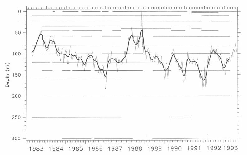
Figure 2. Buoy sampling diagram at 0°, 140°W, showing the history of observations at this location at the various depths sampled. Note that only a few depths have continuous sampling over the 10 years of operation. The overlay of 20°C depth (filtered with a 121-day triangle (dark), and 17-day triangle (light)) shows that this value can be reliably calculated by vertical interpolation with no gaps even though temperature at any of the fixed levels would be gappy.
Pentad averages of twice-daily outgoing longwave radiation (OLR) data observed by satellite were used in this study to estimate the location and strength of tropical deep convection. This data set has been the basis for numerous studies of tropical convective activity, in which low values of OLR are assumed to indicate the presence of tall cumulus towers associated with intense convection [Weickmann et al., 1985; Lau and Chan, 1985; Rui and Wang, 1990; Waliser et al., 1993]. The data are obtained from National Oceanic and Atmospheric Administration's polar-orbiting satellites as radiance measurements in an infrared window channel. The window radiance is then converted to a broad-band estimate of the total outgoing longwave radiation [Gruber and Krueger, 1984]. Global measurements are binned into a day and a night observation on a 2˝° by 2˝° global grid. Missing data occur both in time and space. The data used here have been interpolated in time and then averaged into 73 pentads per year. Chelliah and Arkin [1992] have documented spurious variability in the OLR data due to different satellite equatorial crossing times and different window channel radiometers. These variations are confined to certain regions, especially those having a large diurnal cycle and should have no impact on our results.
Return to previous section or go to next section