U.S. Dept. of Commerce / NOAA / OAR / PMEL / Publications
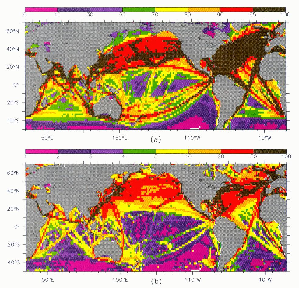
Fig. 1. The distribution of the 1946-1993 COADS SLP data. a) Percentage of months in which each 2 × 2 degree grid point has data. b) Average number of observations used in calculating each monthly mean COADS SLP data point.
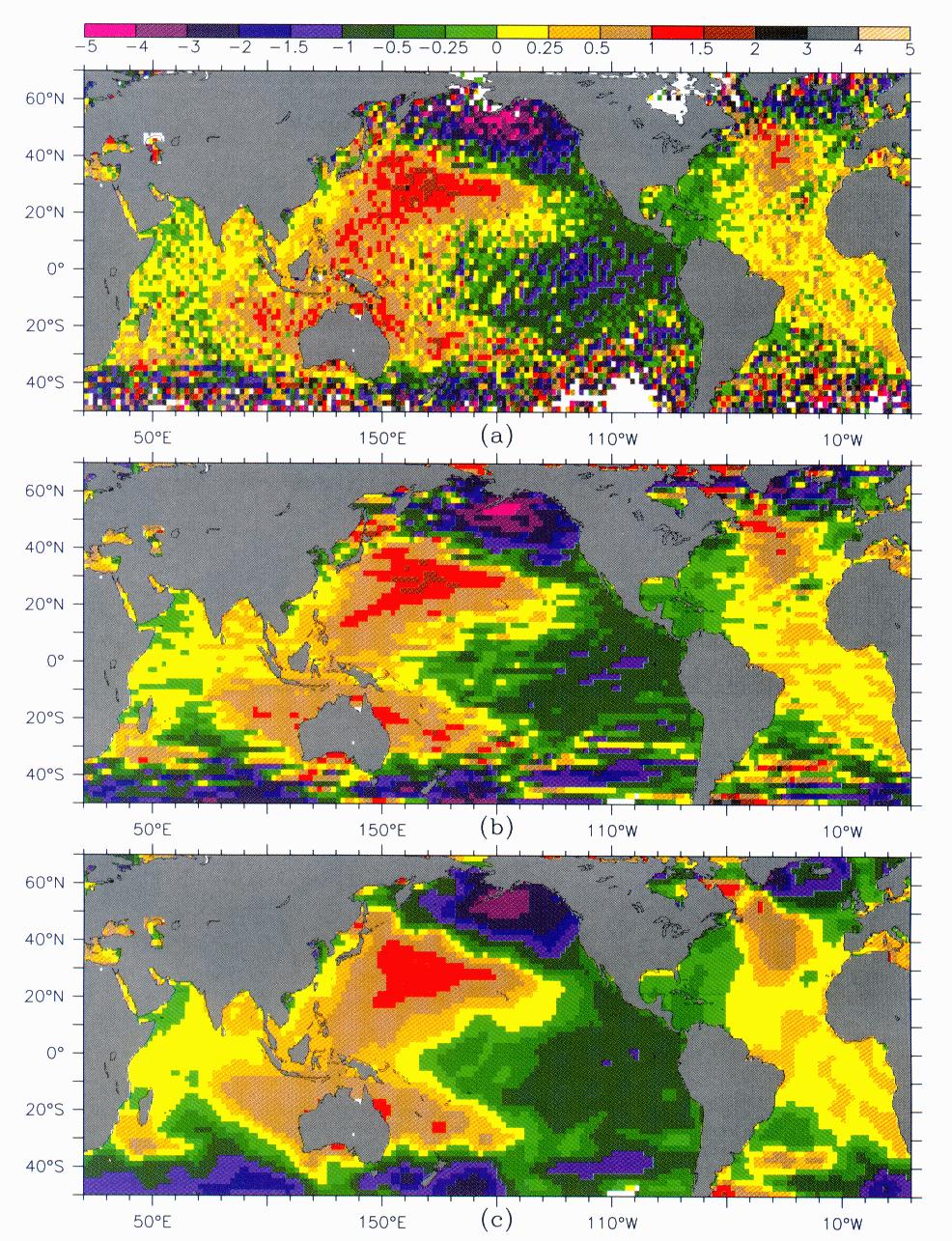
Fig. 2. The December Year(0) SLPA El Nińo composite (see section 4) using different spatial smoothers. a) No spatial smoothing. Note the non-uniform shading intervals, so that variability in the tropics can be seen. b) The same field with gaps filled via linear zonal interpolation, and smoothed via a zonal triangle of ten degree width. c) The same months smoothed by application of the RC smoother (see section 2). All composite results presented hereafter use this latter filling and smoothing.
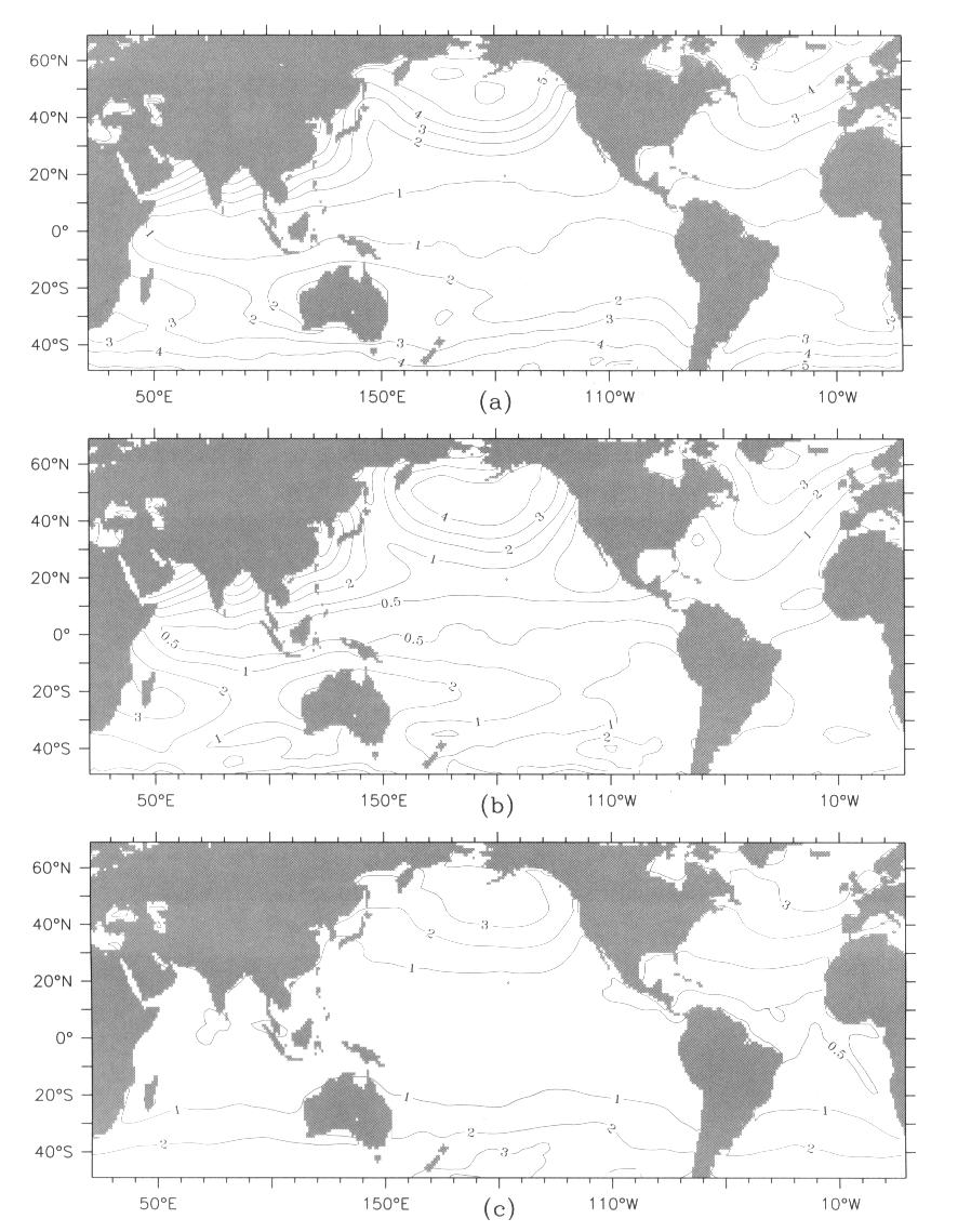
Fig. 3. Standard deviations of the RC smoothed 1946-1993 monthly COADS SLP data. The contour interval is 1 mb with the addition of the 0.5 mb contour to show structure in the tropics. a) standard deviation of SLP over the entire record. b) standard deviation of the monthly mean SLP climatology. c) standard deviation of SLP anomaly (monthly climatology removed) over the entire record.
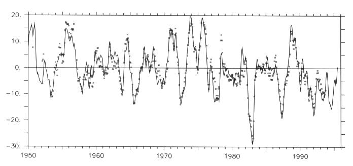
Fig. 4. Troup SOI (solid line) and our COADS "surrogate" of Troup SOI (symbols). Both are shown time smoothed with a 5-month width triangle filter.
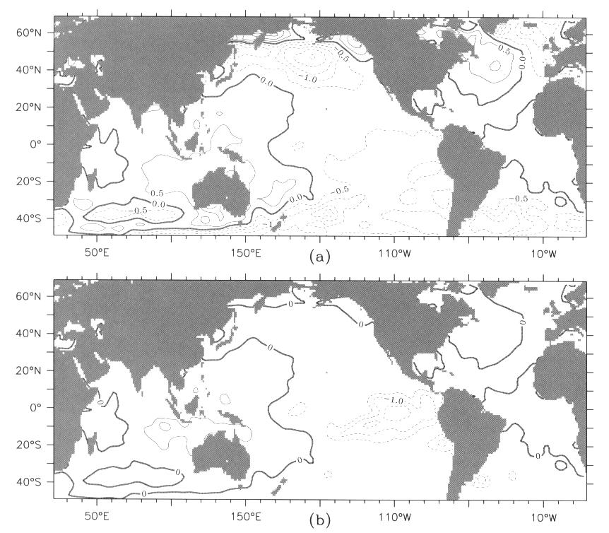
Fig. 5. The effect of normalizing SLPA by Fig. 3c to create SLPAN. Composite September(0) as an example. a) SLPA, contoured every 0.5 mb. b) SLPAN, contoured with zero (heavy line) and then ±0.8, ±1.0, ±1.2, ±1.4, ±1.6, etc... The ±0.8 contours correspond to a local Normal-z 99% significance level. Significance levels of contours are discussed in Section 4.1.
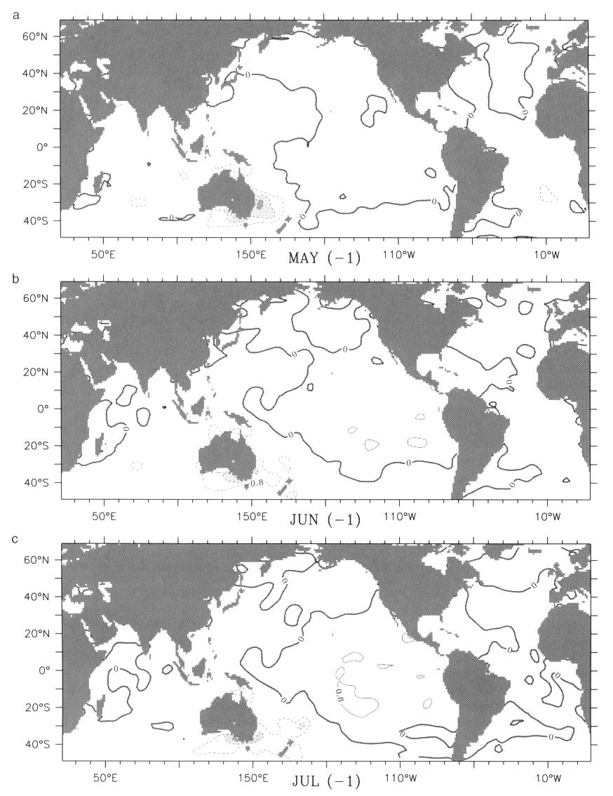
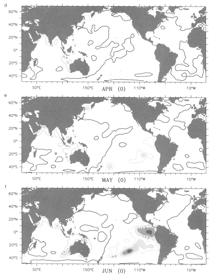
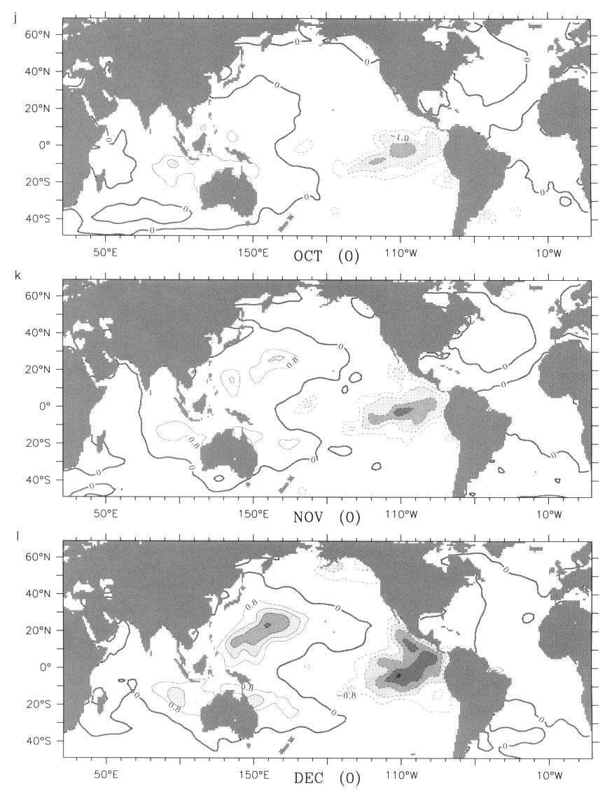
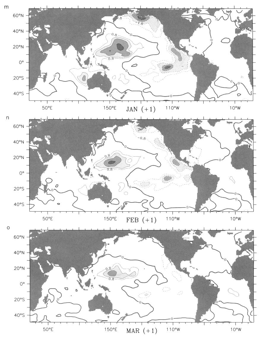
Fig. 6. The evolution of the SLPAN El Nińo composite, May(-1) through July(-1) and April(0) through April(+1). No significant signals are seen between August(-1) and March(0). Contours are as in Fig. 5(b). SLPAN in excess of ±1 is shaded. See Section 4.2 for discussion of composite features.
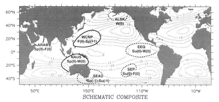
Fig. 7. Schematic representation of the major features of the composite, positive (solid line) and negative (broken line), superimposed on the annual mean SLP field. The boreal seasons for each feature are given, with Sp(-1) = March-April-May of Year(-1), etc. Contours are in (SLP - 1000) mb and the contour interval is 2 mb.
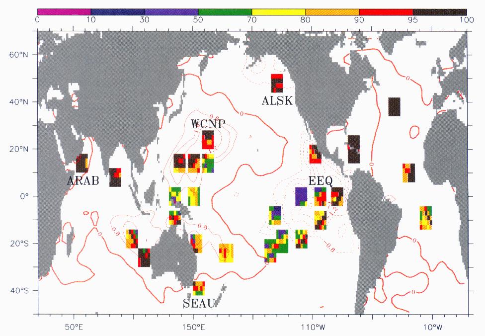
Fig. 8. Location of some of the time series regions used to assess the robustness of the composite, superimposed on December(0) SLPAN. Regions whose time series plots are presented in Section 5 are labeled. Coloration indicates the percentage of months with data as in Fig. 1a.
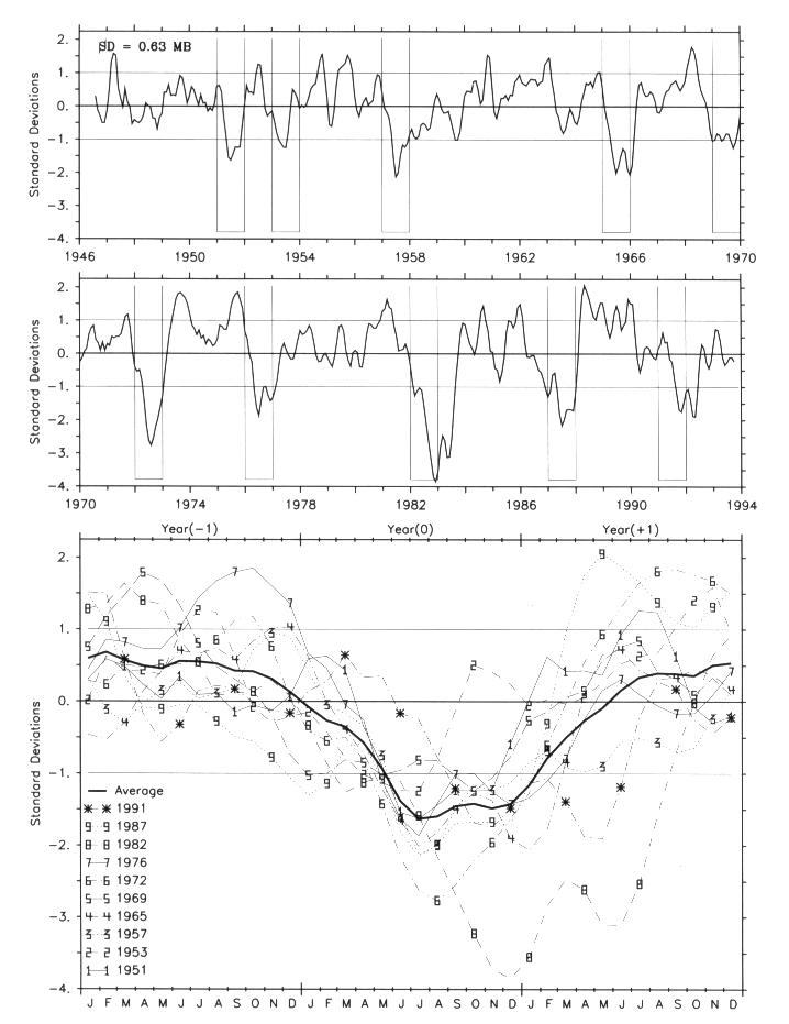
Fig. 9. The EEQ SLPAN time series averaged over 108°W to 98°W, 4°S to 4°N and time smoothed by a 5-mo triangle filter (see section 5). The top two panels present the time series, 1946-1993. Bottom brackets identify each ENSO Year(0) . The bottom panel presents an overlay of SLPAN for each ENSO period from Year(-1) to Year(+1). The different ENSO events are indicated by number: 1 = 1951, 2 = 1953, 3 = 1957, 4 = 1965, 5 = 1969, 6 = 1972, 7 = 1976, 8 = 1982, 9 = 1987, * = 1991.
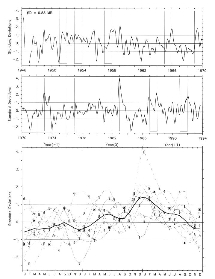
Fig. 10. Same as Fig. 9, except for the WCNP region, 158° to 168°E, 20° to 28N°.
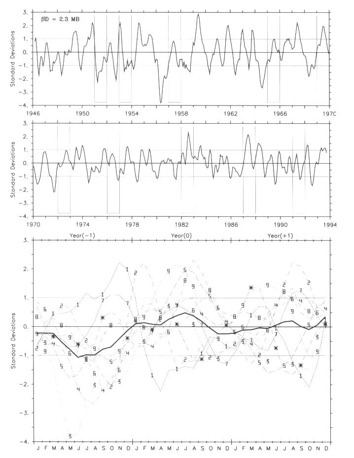
Fig. 11. Same as Fig. 9, except for the SEAU region, 150° to 160°E, 42° to 36°S.
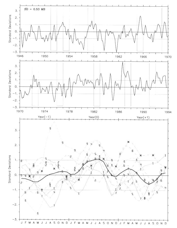
Fig. 12. Same as Fig. 9, except for the ARAB region, 52° to 62°E, 10° to 18°N.
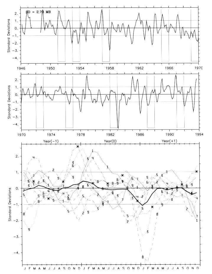
Fig. 13. Same as Fig. 9, except for the ALSK region, 144° to 134°W, 44° to 52°N.
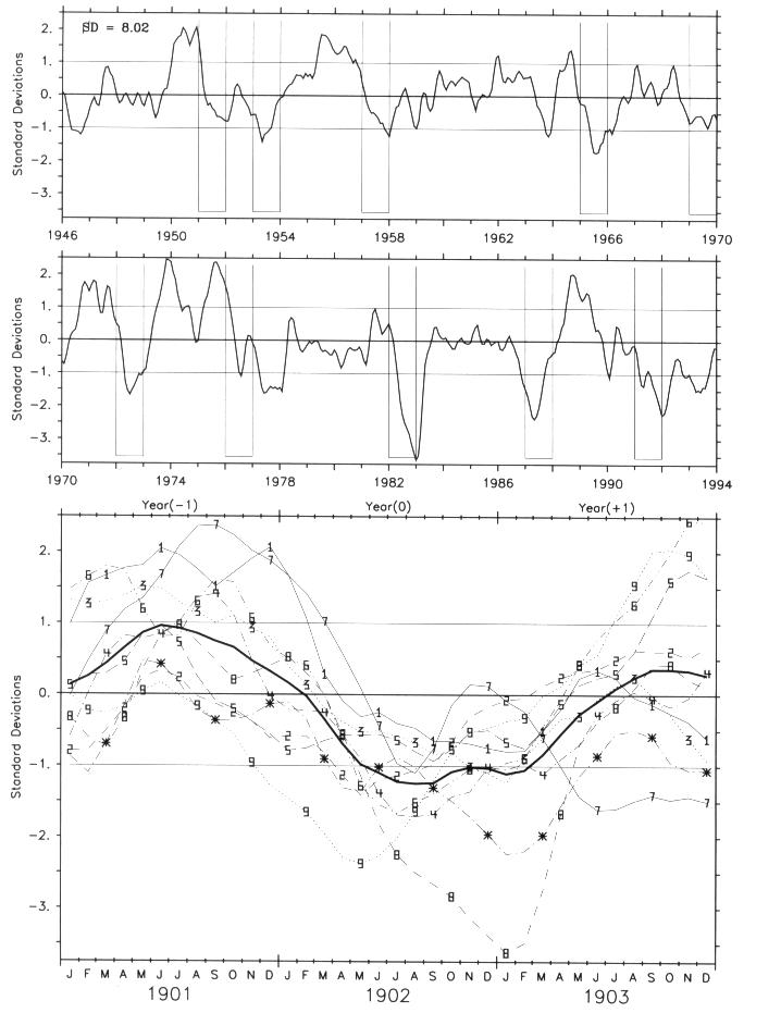
Fig. 14. Same as Fig. 9, except for the Troup SOI, smoothed and normalized as in Figs. 9-13. See section 5.
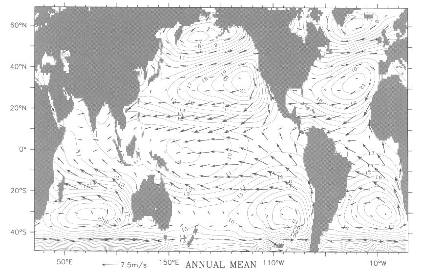
Fig. A1. The annual average SLP and wind fields, RC smoothed. SLP is shown as (SLP - 1000) mb with a contour interval of 1 mb. The annual average wind field is superimposed (scale as indicated).
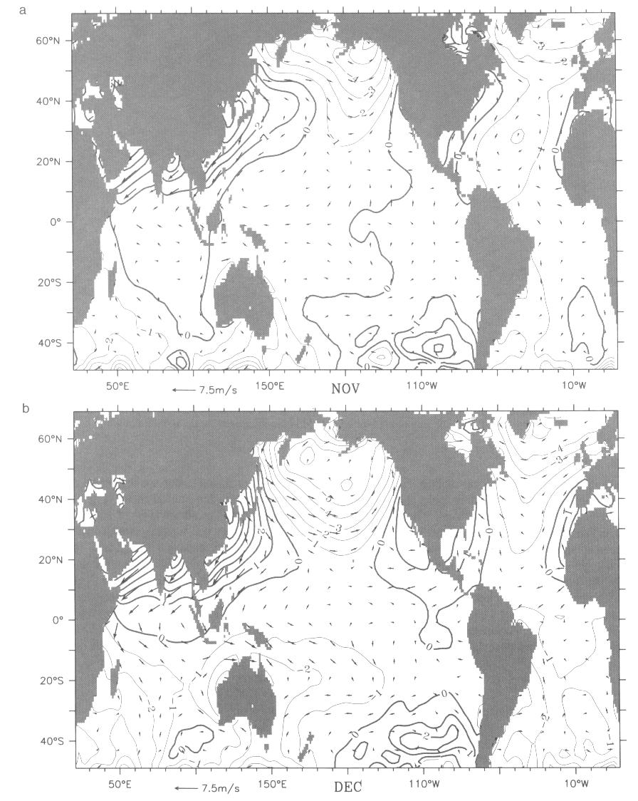
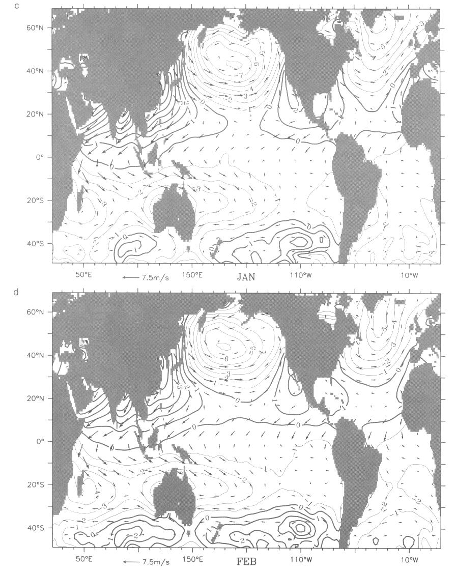
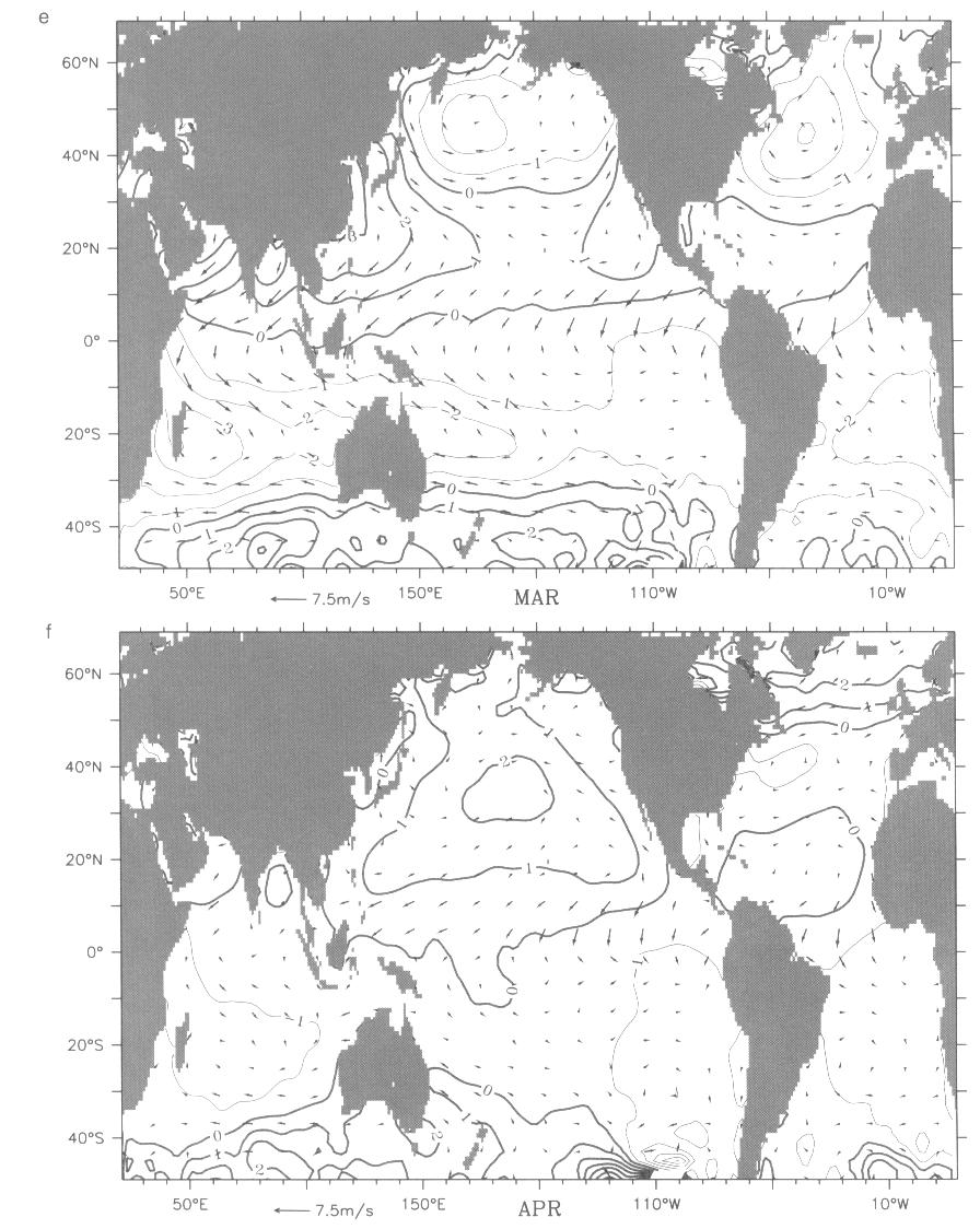
Fig. A2. The SLP and wind monthly climatology departure from their annual means, RC smoothed. The SLP departure in mb, positive (heavy line) and negative (light line). The wind departure with scale as indicated.
Table 1. Correlations between surrogate and station time series.
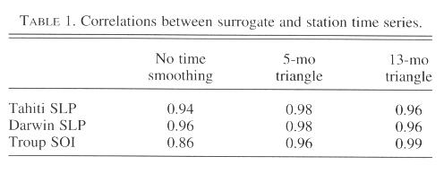
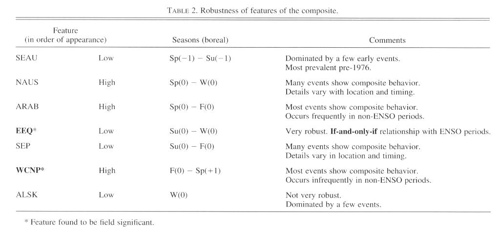
Table 2. Robustness of features of the composite.
Return to previous section or go back to Abstract