Near-surface shear in the Pacific cold tongue front at 2°N, 140°W was measured using a set of five moored current meters between 5 and 25 m for nine months during 2004–05. Mean near-surface currents were strongly westward and only weakly northward (~3 cm s-1). Mean near-surface shear was primarily westward and, thus, oriented to the left of the southeasterly trades. When the southwestward geostrophic shear was subtracted from the observed shear, the residual ageostrophic currents relative to 25 m were northward and had an Ekman-like spiral, in qualitative agreement with an Ekman model modified for regions with a vertically uniform front. According to this "frontal Ekman" model, the ageostrophic Ekman spiral is forced by the portion of the wind stress that is not balanced by the surface geostrophic shear. Analysis of a composite tropical instability wave (TIW) confirms that ageostrophic shear is minimized when winds blow along the front, and strengthens when winds blow oblique to the front. Furthermore, the magnitude of the near-surface shear, both in the TIW and diurnal composites, was sensitive to near-surface stratification and mixing. A diurnal jet was observed that was on average 12 cm s-1 stronger at 5 m than at 25 m, even though daytime stratification was weak. The resulting Richardson number indicates that turbulent viscosity is larger at night than daytime and decreases with depth. A "generalized Ekman" model is also developed that assumes that viscosity becomes zero below a defined frictional layer. The generalized model reproduces many of the features of the observed mean shear and is valid both in frontal regions and at the equator.
Away from the equator, the earth's rotation causes the net wind-forced response to be to the right (left) of the wind in the Northern (Southern) Hemisphere. Consequently, trade wind forcing in the tropics tends to drive a divergent "Ekman" meridional transport that causes upwelling on the equator. Although there have been several studies that estimate the poleward Ekman and equatorward geostrophic transports of the meridional overturning cell (Wyrkti 1981; Bryden and Brady 1985; Johnson et al. 2001; Meinen et al. 2001; Kug et al. 2003), there have been few direct measurements of their structure. In particular, most of these measurements have relied either upon shipboard (e.g., Johnson et al. 2001; Wijffels et al. 1994) or moored (e.g., Halpern and Freitag 1987; Weisberg and Qiao 2000) acoustic Doppler current profilers (ADCPs), neither of which observe the velocity profile within the top 25 m, precisely where the wind-driven poleward flow is expected to be largest. In this poorly defined situation, some analyses of the meridional overturning cell have assumed a constant shear within the surface layer (e.g., Johnson et al. 2001; Weisberg and Qiao 2000), while others have assumed a slab layer (e.g., Wijffels et al. 1994). Because the zero crossing of meridional velocity is relatively shallow, these differing assumptions have a profound effect upon the estimated net transport. Thus, in this paper, we ask the question: Is there shear within the off-equatorial near-surface mean poleward flow? To address this, from May 2004 through February 2005, a test mooring near the 2°N, 140°W TAO mooring was instrumented with five current meters in the top 25 m.
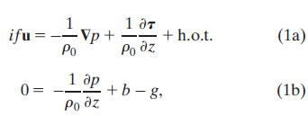
We will consider the most basic framework for interpreting near-surface currents at 2°N: the linear, steady-state equations of motion in hydrostatic balance:
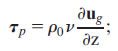
where i is ![]() , u is the horizontal velocity vector, f is the vertical component of the Coriolis parameter, ρ0 is the background density, ∇ is the horizontal gradient operator, p is pressure, g is gravity, and b = g(ρ0 − ρ)/ρ0 is buoyancy. Here h.o.t. refers to higher-order terms (e.g., horizontal eddy stress terms), which, for simplicity, we assume to be negligible. We then make the standard assumptions that the stress vector within the fluid, τ(z), can be related to the shear profile through a turbulent viscosity parameter ν,
, u is the horizontal velocity vector, f is the vertical component of the Coriolis parameter, ρ0 is the background density, ∇ is the horizontal gradient operator, p is pressure, g is gravity, and b = g(ρ0 − ρ)/ρ0 is buoyancy. Here h.o.t. refers to higher-order terms (e.g., horizontal eddy stress terms), which, for simplicity, we assume to be negligible. We then make the standard assumptions that the stress vector within the fluid, τ(z), can be related to the shear profile through a turbulent viscosity parameter ν,
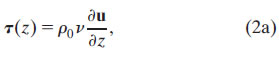
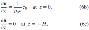
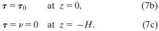
and that, at the surface, the shear stress balances the wind stress, τ0:
The bottom boundary condition for (1) is less straight-forward, as will be discussed.
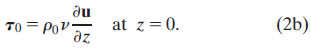
At depths where both ν = 0 and ∂ν/∂z = 0, the flow is inviscid and (1a) reduces to the geostrophic balance. Because depth variations in the pressure gradient can be related to the buoyancy gradient by (1b), the geostrophic shear is parallel to density contours and is referred to as "thermal wind shear":
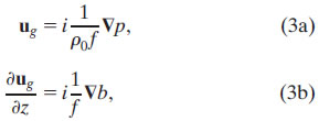
where ug is the geostrophic velocity. Near 2°N in the eastern and central Pacific, a strong temperature front exists between the cold water upwelled at the equator and the warm water advected east by the North Equatorial Counter Current. We therefore expect strong thermal wind shear oriented along this front.
Away from the equator and in regions with no fronts, that is, where the shear is entirely ageostrophic, the stress divergence effects can be separated from the pressure gradient by decomposing the velocity in (1a) into geostrophic and ageostrophic components (u = ug + ua ). Following Ekman (1905), Eq. (1a) can be further simplified by assuming that viscosity is vertically uniform. Invoking the standard top boundary condition that surface shear is proportional to the wind stress (2b) and making a no-drag bottom boundary condition, the "classical Ekman" model for the ageostrophic velocity profile then becomes
classical Ekman: 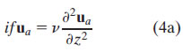
with boundary conditions:
where H is some depth below the frictional layer, functionally set as ∞.
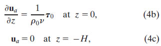
We now consider the Ekman response in frontal regions. Above the top of the thermocline (roughly 125 m at 2°N, 140°W), vertical mixing likely causes the subsurface frontal structure to be similar to the surface. Within the thermocline, though, the horizontal temperature gradient probably differs from the sea surface temperature (SST) gradient. For simplicity and because we lack more detailed information, we will assume that the buoyancy front within the upper ocean is vertically uniform and equivalent to the surface front. By (3b), this implies that the geostrophic shear is also vertically uniform and therefore does not enter the stress divergence term on the rhs of (1a). Equation (1a) thus reduces to
Ekman uniform front:
which is identical to the classical Ekman model (4a). The vertically uniform geostrophic shear, however, will contribute to the top boundary condition (2b), which can be rearranged to be a boundary condition for the ageostrophic profile:
where, as in (4), viscosity is assumed to be vertically uniform. The bottom boundary condition (5c) states that the influence of the wind dies out by z = −H, and at that level the flow is geostrophic. Note that the "frontal Ekman" model (5) resembles the classical Ekman model (4), with the important distinction that the effective surface stress τeff that forces the ageostrophic Ekman spiral is only a portion of the wind stress—the portion that is out of balance with the surface geostrophic shear stress
that is, τeff = τ0 − τp. In other words, in a region with a vertically uniform front, the ageostrophic Ekman spiral is a linear sum of the classic response to the wind stress τ0 and a second spiral forced by −τp. This second ageostrophic spiral counterbalances the surface geostrophic shear associated with the front, assuring that the total surface shear satisfies the boundary condition (2b).
Because the geostrophic shear depends on the factor 1/f, the stress contribution from a given surface density gradient is larger in tropical regions than at higher latitudes. At the equator, however, geostrophic shear is undefined. As shown by Stommel (1960), on the equator, the zonal wind stress tends to balance the zonal pressure gradient. Assuming steady, linear, homogenous flow, with uniform viscosity, Stommel determined an analytic solution for p and u that satisfied
Stommel model: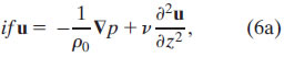
with boundary conditions:
in addition to eastern and western boundary conditions on the zonal transport. Unlike the Ekman "no-drag" bottom boundary condition, the Stommel bottom boundary condition (6c) requires that the shear (and thus stress) is zero at the fixed level z = − H, nominally set as the center of the Equatorial Undercurrent (EUC). The resulting solution is valid both on and off the equator and reproduces many of the features of the equatorial current system including a South Equatorial Current lying above an EUC.
Fronts, however, are a ubiquitous feature of the global oceans, and the assumption in the original Stommel model that density gradients are negligible is one of its major limitations. The Stommel model was extended to include fronts by Schneider and Müller (1994), and Bonjean and Lagerloef (2002, hereafter referred to as BL02) derived an analytical solution for the vertical shear in the extended Stommel model. Both derivations assume vertically uniform fronts and vertically uniform viscosity. In particular, the analytical solution for the shear enabled BL02 to determine the effects of mixing at 30 m on the upper 30-m layer currents (which are given a nominal depth of 15 m). To map the global 15-m currents, BL02 estimate viscosity from wind speed based upon the Santiago-Mandujano and Firing (1990) empirical relationship, determine the buoyancy gradient from the Tropical Rainfall Measuring Mission (TRMM) Microwave Imager (TMI) SST, and the surface pressure gradient and wind stress from satellite altimetry and scatterometer fields. The resulting 15-m velocity product is referred to as the Ocean Surface Current Analyses—Real time (OSCAR) and is available online at www.oscar.noaa.gov).
While the boundary conditions (6b)–(6c) invoked by Stommel (1960) have become widely used, they are not always realistic. Stommel notes that, while the zero shear bottom boundary condition (6c) is satisfied at the center of the EUC, the EUC shoals to the east and therefore the no-stress level is not strictly flat. Likewise, poleward of the EUC, the shear is not generally zero at this depth (e.g., the thicker South Equatorial Currents flank the EUC). This is particularly a problem for the BL02 formulation that assumes vertically uniform fronts and thus vertically uniform geostrophic shears (3b). In this case, the zero total shear bottom boundary condition (6c) implicitly requires an ageostrophic shear at z = −H that is equal and opposite to the thermal wind component. BL02 argued that the shear solution at 30 m is relatively insensitive to H and chose H based upon a best-fit procedure to be 70 m for the OSCAR product. In contrast, the Ekman frontal model (5) allows the flow to transition to geostrophic flow at H, but has a singularity at the equator.
The conundrum can be resolved if the viscosity decays with depth so that, at the base of the frictional layer, the stress becomes zero, while the shear can remain nonzero. This assumption is consistent with microstructure measurements (e.g., Peters et al. 1988; Smyth et al. 1996) that show a several decade reduction in viscosity between the surface mixed layer and deeper thermocline values. An equation for the stress can then be derived by taking the vertical derivative of (1) and expressing shear in terms of the stress (2a):
generalized Ekman: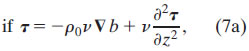
As in the classical Ekman model (4) and frontal Ekman model (5), viscosity and buoyancy gradient profiles are prescribed. The buoyancy gradient in (7a), however, is not required to be vertically uniform, so this "generalized Ekman" model (7) is valid for regions in which the front is tilted. Furthermore, because f does not appear in the denominator of (7), the generalized Ekman model is also valid both on and off the equator. With viscosity and buoyancy gradient profiles known or assumed, (7) can be solved numerically for τ, and the stress–shear relationship (2a) can then be used to determine the shear flow profile. The shear can then be decomposed into geostrophic and ageostrophic components according to (3b).
Finally, it is worth considering the effect of these assumptions on the geostrophic and ageostrophic (Ekman) transport. By vertically integrating (1a) from the surface to the depth −H, the transport U can be expressed as
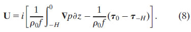
The first term on the rhs of (8) is the geostrophic transport; the last two terms are the ageostrophic Ekman transport associated with the surface wind stress (τ0) and with the stress at the base of the frictional layer (τ−H). A front modifies the total transport in the direction of the front through the geostrophic term and potentially modifies the transport perpendicular to the front through the Ekman transport associated with τ−H. In particular, if, as in the case of the frontal Ekman model (5), the viscosity is not zero at the depth −H and a thermal wind shear exists at that depth, then τ−H will be nonzero and will induce an ageostrophic Ekman transport in the direction of the density gradient, that is, perpendicular to the front. However, if viscosity tapers to zero at depth −H, as in the generalized Ekman model (7), then the net Ekman transport is to the right of the wind and invariant to the front. The Ekman transport in the generalized Ekman model is thus identical to that in the classical Ekman model (4) and differs from the frontal Ekman model transport. Since the generalized and frontal Ekman models differ primarily in their bottom boundary conditions, it is likely that their differences are most apparent in the lower portion of their Ekman spirals.
The remainder of this paper will explore the consequences of the two principal mechanisms by which a vertically uniform front affects the near-surface currents: First, through the surface boundary condition (2b), in which the geostrophic shear contributes to the total surface shear ∂u/∂z, thereby modifying the effective stress that forces the ageostrophic flow, and second, through the front's geostrophic interior shear that is added to the ageostrophic Ekman spiral. If the front is tilted, then additional possibilities arise, which cannot be evaluated from the single mooring studied here. Nevertheless, as we will show, even a simple vertically uniform front produces systematic changes in the magnitude and direction of the near-surface currents. In the region of the cold tongue front, near-surface flow lies within the poleward branch of the tropical Pacific meridional overturning cell. The consequences of the front, therefore, can include modifying the large-scale overturning circulation.
After the conclusion of the Eastern Pacific Investigation of Climate Processes (EPIC) experiment (Cronin et al. 2002), five current meters were available for an opportunistic study of near-surface shear. To quantify the near-surface shear in the poleward branch of the meridional overturning cell, the study needed to be off the equator and at a longitude that had strong equatorial upwelling and a well-developed cold tongue during boreal fall. A NOAA/Pacific Marine Environmental Laboratory (PMEL) Engineering Development Division test mooring scheduled for deployment near the 2°N, 140°W Tropical Atmosphere Ocean (TAO) mooring in May 2004 satisfied these requirements and was available for this study.
The test mooring carried a wind sensor, a sea surface temperature module at 1-m depth, and five Sontek current meters that measured horizontal currents in 1-m bins at 5 m, 10 m, 15 m, 20 m, and 25 m. Sontek current meters measure currents at a 1-Hz rate for 2 min every 20 min. Speed and direction resolution are 0.1 cm s-1 and 0.1°, with nominal accuracy of ±5 cm s-1, and ±5° for daily-averaged data, although current meters above 80 m appear to be more accurate than this (Freitag et al. 2003). Each Sontek current meter was mounted with a TAO temperature module that had a thermistor 3.3 m below the center of the current meter bin (i.e., at 8.3 m, 13.3, 18.3, 23.3, and 28.3 m). The TAO sea surface temperature module has an accuracy of 0.03°C, while subsurface modules have an accuracy of 0.09°C (Freitag et al. 1994).
Linear trends between pre- and postcalibrations were applied to all temperature data. Based upon the post-calibrations and intercomparisons with the other sensors, it appeared that the 25-m current meter and the 23.3-m thermistor had unacceptable calibration drifts. Thus, the 23.3-m thermistor data are not used in this analysis. Inspection of the 25-m current meter compass pitch and roll data showed that the quality deteriorated abruptly on 8 October 2004. Thus, for analysis of the mean shear and the influence of the diurnal cycle, we focus on the period in which all five current meters were functioning (24 May–7 October 2004). Shears during this period are computed by referencing the velocity at each level to the velocity at 25 m. This was deemed more robust than taking differences between each 5-m interval. Because the 25-m Sontek malfunctioned during the period of strong tropical instability waves (TIWs), currents were referenced to 20 m for the TIW shear analysis (from 1 November 2004 to 28 February 2005).
Wind stress was estimated using the Coupled Ocean–Atmosphere Response Experiment (COARE) version 3 bulk algorithm (Fairall et al. 2003). This algorithm requires not only wind speed and direction estimates relative to the ocean surface, but also measurements of the air and sea surface temperature and surface specific humidity. Although the test mooring carried a wind sensor, it did not carry an air temperature and relative humidity sensor. Thus, wind stress was calculated using hourly data from the 2°N, 140°W TAO mooring that was 6 n mi away from the test mooring.
To estimate the temperature gradient, we use version 4 TMI SST data obtained from the Asia–Pacific Data Research Center (APDRC) data delivery site (see online at http://apdrc.soest.hawaii.edu/data/data.php). The APDRC TMI daily fields are 3-day running means on a 0.25° × 0.25° spatial grid. Because the buoy temperature at 28.3 m nearly always differs from the 1-m SST by less than 0.2°C, the top 25 m can be considered well mixed for this purpose and we assume that the TMI SST gradients represent the horizontal gradients of temperature within the top 25 m. Geostrophic thermal wind is expected to respond slowly to changes in the horizontal temperature field and the Rossby radius of deformation at 2°N is roughly 210 km. Thus, the TMI data were filtered with a 5-day low-pass filter and the horizontal gradients were computed by fitting a straight line to the SST over eight grid points (i.e., 222 km).
To compute the geostrophic component of the near-surface shear (3b), we assume that the buoyancy gradient can be estimated from the temperature gradient. However, the temperature front on the northern edge of the cold tongue is collocated with a strong salinity front separating the freshwater beneath the intertropical convergence zone from the upwelled cool, salty equatorial water (Ando and McPhaden 1997; McPhaden et al. 2008). Covariations of daily-averaged SST and sea surface salinity (SSS) measurements at the nearby 2°N, 140°W TAO buoy over the period in which all five current meters functioned had a correlation of −0.74 and a mean slope (dS/dT) of −0.018 psu K−1. Thus, with a thermal expansion coefficient α = 3.0 × 10⁻⁴ K−1, and a haline contraction coefficient of 7.4 × 10⁻³ psu−1 (both of which are based upon the equation of state for mean surface conditions at 2°N, 140°W), the effective thermal expansion coefficient is estimated as αeff = α − β dS/dT ∼ 4.3 × 10⁻⁴ K−1 and the buoyancy gradient in (3b) is then estimated as ∇b = gαeff ∇T. During the TIW period (1 November 2004–28 February 2005), co-variations of coincident SST and SSS daily measurements were less correlated (−0.3) and the effective thermal expansion coefficient was estimated to be 3.4 × 10⁻⁴ K−1.
With the geostrophic shear estimated from the TMI SST, the observed mean total currents relative to 25 m are decomposed into geostrophic and residual ageostrophic components for the period during which all five current meters functioned (24 May–7 October 2004). The standard error for the mean shear is estimated as the standard deviation divided by the square root of the degrees of freedom. The integral time scale for the currents relative to 25 m, estimated as the integral of the temporal autocorrelation function, was found to be about 2 days. Thus, the mean shear computed over the 136-day period had approximately 68 degrees of freedom.
The resulting ageostrophic currents relative to 25 m are then compared to simulations by the classical Ekman model (4), the frontal Ekman model (5), and the generalized Ekman model (7). A novel result of this study is that the ageostrophic Ekman currents depend, not only upon the wind, but also upon the strength and orientation of the front relative to the wind. Observations during the passage of tropical instability waves (Willett et al. 2006) offer an opportunity to test this idea since the orientation of the front varies over the course of a wave, while the orientation of the wind is relatively steady.
To compute a composite TIW, an index was created using complex demodulation on the SST for a 30-day periodicity. Complex demodulation (Bloomfield 1976) is a type of bandpass that represents a time series as a near sinusoid with time-varying amplitude and phase that is equivalent to allowing slow frequency variation. It is thus appropriate for a nearly periodic signal whose variability wanders within the frequency band. The complex demodulation phase of buoy SST provided a good index of the TIW signal and was used as the basis for compositing the other quantities (currents, currents relative to 20 m and their geostrophic and agoeostrophic components, winds, and temperature). All variables were decomposed using complex demodulation around a central period of 30 days for the period when TIW were prominent in the record, 1 November 2004–28 February 2005. The near-sinusoidal representation of these were binned according to the concurrent SST phase to create a 30-day composite.
Shear is also expected to be sensitive to viscosity. Because stratification and mixing have their largest variations over the diurnal cycle, while wind and frontal forcing have much weaker or negligible variations at this time scale, the effects of viscosity on shear can essentially be isolated from other processes by considering the composite diurnal cycle. To compute diurnal composites of wind, temperature, and velocity, the time series over the 4.5-month period when all five current meters were available were binned into local time of day and then averaged.
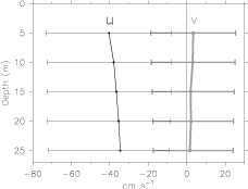
Fig. 1. The mean zonal (black) and meridional (gray) currents (cm s−1) at 2°N, 140°W with ±1 standard deviation indicated at 5, 10, 15, 20, and 25 m, computed for the period 24 May–7 Oct 2004.
The mean flow above 25 m was primarily westward, with a very weak poleward component, for the period 24 May–7 October 2004 (Fig. 1). The mean westward component was 41 cm s−1 at 5 m, decreasing to 35 cm s−1 at 25 m, while the mean poleward component was only 3.3 cm s−1 at 5 m, decreasing to 1.6 cm s−1 at 25 m. For the full period 24 May 2004–28 February 2005, the mean westward currents above 20 m were stronger by ∼15 cm s−1, but the poleward currents were still under 4 cm s−1 (not shown).
Observed poleward currents and shear were substantially weaker than the 6 cm s−1 currents at 20 m and (2 cm s−1)/10-m poleward shear at 25 m found at 2°N by Johnson et al. (2001) from nine years of shipboard ADCP data between 95° and 170°W. Based upon this shear, Johnson et al. extrapolated the shipboard ADCP measurements to the surface to estimate a 10 cm s−1 poleward surface current at 2°N (about 3 times larger than we observed). Our observed weak poleward currents at 2°N, 140°W are even more curious when one considers the implications for the meridional overturning cell transport. Estimates of equatorial upwelling made over the two decades since Wyrtki (1981) have ranged from 30 Sv (Meinen et al. 2001) to 60 Sv (Sv ≡ 106 m3 s−1) (Johnson et al. 2001), the great majority of which must occur equatorward of 2° latitude. Likewise, because 140°W is a central longitude within the cold tongue system, where easterly trades are near their maximum, one might expect 140°W to have larger poleward currents than the zonal average and thus the implied transport to be an upper bound estimate. However, the measured poleward currents at 2°N, 140°W, if representative of the currents across the 80° longitude of the cold tongue, imply a poleward transport of only 7 Sv. With a similar transport assumed for the Southern Hemisphere, the implied equatorial upwelling transport is only 14 Sv, less than half of the lowest estimate. Winds during the study period were not anomalous compared to climatology (not shown). It is possible that at the cold tongue front a local minimum in the near-surface poleward currents exists that is not resolved in the Johnson et al. (2001) mean section owing to the considerable temporal, meridional, and zonal averaging done in that analysis. If this local minimum feature is real, then what causes it? What happens to the poleward branch of the tropical cell at the front? What physics control the structures of zonal and meridional shear?
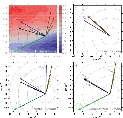
Fig. 2. Vectors of the 2°N, 140°W mean wind (blue) and currents relative to 25 m (black) with their geostrophic (green) and ageostrophic (brown) components, as (a) observed for the period 24 May–7 Oct 2004 and as simulated by the (b) classical, (c) frontal, and (d) generalized Ekman models. The wind shown in (a) is the vector wind speed and in (b)−(d) is the wind stress vector. The surface geostrophic stress (τp = ρ0ν ∂ug/∂z) and effective wind stress (τeff = τ0 − τp) are also shown in (c). The magnitudes of the wind and relative currents are indicated by the circles. Units for the relative currents are cm s−1, m s−1 for wind speed, and 10−2 N m−2 for wind stress. Currents at 5, 10, 15, and 20 m, relative to 25 m, can be distinguished by their decreasing amplitude. Standard errors are indicated by the ellipses on the arrow heads. The vectors in (a) are superimposed upon the mean TMI SST field.
Because the observed poleward shear is so weak, the mean currents relative to 25 m are nearly westward and thus, surprisingly, are to the left of the mean winds (Fig. 2a). The 2°N, 140°W site, however, is in the cold tongue front, with warm water to the north and west, and therefore the observed shear has a geostrophic component that is southwestward, parallel to the SST contours. When the geostrophic shear is subtracted from the observed currents, the residual ageostrophic currents relative to 25 m are predominantly northward and have the appearance of an Ekman spiral (Fig. 2a). In particular, the 5-m ageostrophic current referenced to 25 m is oriented 71° to the right of the wind, and at each subsequent depth the ageostrophic current referenced to 25 m is weaker and tends to be oriented to the right of the ageostrophic currents above.
If the observed ageostrophic spiral is interpreted as a classical Ekman spiral forced by the wind stress (4), then the orientation of the 5-m ageostrophic current relative to 25 m would suggest that the reference depth of 25 m is near the e-folding ''Ekman depth,'', ![]() , (for a classical Ekman spiral, the ageostrophic current has a 1/e decay in magnitude and rotates by 1 rad at this depth). For 2°N, this would imply that the viscosity (ν) was ∼ 1.6 × 10⁻³ m2 s−1. By (4b), though, this would imply that the mean wind stress of 0.07 N m−2 should cause a shear of ∼(0.45 m s−1)(20 m)−1, more than an order of magnitude larger than observed. On the other hand, all Ekman models discussed in sections 1 and 2, (4)–(7), assume that the wind stress balances the surface shear stress according to (2b). Thus for our analysis, we determine ν from (2b) with the surface shear estimated from the mean 5- and 15-m currents. The resulting viscosity is an order of magnitude larger—roughly 16 × 10−3 m2 s−1. While this viscosity is quite a bit larger than that given by the Santiago-Mandujano and Firing (1990) relation (5 × 10⁻³ m2 s−1), other studies (F. Bonjean 2008, personal communication) have also found that the Santiago-Mandujano and Firing (1990) viscosity appear to be biased low. With ν set as 16 × 10−3 m2 s−1, the Ekman depth is ∼80 m and the ageostrophic shears above 25 m resulting from the classical Ekman model more closely parallel the wind stress (Fig. 2b). As a consequence, the observed near-surface shears cannot be reproduced as a linear combination of thermal wind shear plus classical Ekman spiral shear.
, (for a classical Ekman spiral, the ageostrophic current has a 1/e decay in magnitude and rotates by 1 rad at this depth). For 2°N, this would imply that the viscosity (ν) was ∼ 1.6 × 10⁻³ m2 s−1. By (4b), though, this would imply that the mean wind stress of 0.07 N m−2 should cause a shear of ∼(0.45 m s−1)(20 m)−1, more than an order of magnitude larger than observed. On the other hand, all Ekman models discussed in sections 1 and 2, (4)–(7), assume that the wind stress balances the surface shear stress according to (2b). Thus for our analysis, we determine ν from (2b) with the surface shear estimated from the mean 5- and 15-m currents. The resulting viscosity is an order of magnitude larger—roughly 16 × 10−3 m2 s−1. While this viscosity is quite a bit larger than that given by the Santiago-Mandujano and Firing (1990) relation (5 × 10⁻³ m2 s−1), other studies (F. Bonjean 2008, personal communication) have also found that the Santiago-Mandujano and Firing (1990) viscosity appear to be biased low. With ν set as 16 × 10−3 m2 s−1, the Ekman depth is ∼80 m and the ageostrophic shears above 25 m resulting from the classical Ekman model more closely parallel the wind stress (Fig. 2b). As a consequence, the observed near-surface shears cannot be reproduced as a linear combination of thermal wind shear plus classical Ekman spiral shear.
Alternatively, according to the frontal Ekman model (5), the ageostrophic Ekman spiral responds only to that portion of the wind stress that is not balanced by the geostrophic shear (τeff = τ0 − ρ0ν∂ug/∂z). As shown in Fig. 2c, with viscosity set as 16 × 10−3 m2 s−1, the stress associated with the surface geostrophic shear (τp = ρ0ν∂ug/∂z) is slightly larger in magnitude than the wind stress and is oriented to the southwest while the wind stress is oriented to the northwest. Thus, the net effective stress (τeff) forcing the surface ageostrophic shear is roughly northward. The resulting frontal Ekman model ageostrophic currents relative to 25 m are in good agreement with the observed residual ageostrophic currents. Furthermore, when thermal wind is added to the modeled ageostrophic currents, the resulting total currents relative to 25 m are to the left of the wind stress as observed.
As discussed in the introduction, a perhaps more realistic model of the near-surface shear is the generalized Ekman model (7) in which viscosity decays with depth to zero at z = −H. The difficulty of testing this model is that we do not know what the n profile is, nor at what depth it goes to zero, nor what the profile of the buoyancy gradient is. Furthermore, the deepest current observations are at 25 m and the primary differences between the frontal and generalized Ekman models are likely to be below this depth. For simplicity and because the Peters et al. (1988) turbulence measurements indicate that viscosity decays exponentially with depth, we assume viscosity has the form:
ν = A exp(z/D) − B.
It is beyond the scope of this paper and dataset to do a full sensitivity analysis of the parameter space. We therefore arbitrarily set D to be the top of the thermocline (125 m) and choose A and B so that the viscosity is equivalent to 16 × 10−3 m2 s−1 at 10-m depth and zero at the arbitrary depth of 250 m (twice the decay scale). Likewise, for simplicity, we assume that the front is uniform within the frictional layer above 250 m. The resulting generalized Ekman model (Fig. 2d) produces currents relative to 25 m that are to the left of the wind, similar to the results of the frontal Ekman model (Fig. 2c) and to the observations (Fig. 2a).
Although total currents relative to 25 m predicted by both the frontal and generalized Ekman models show some indication of rotation to the left with depth, the observed currents relative to 25 m do not. The standard error (shown as ellipses around the vector heads in Fig. 2a) suggests that this wobble is real. This error, however, does not include any systematic biases and therefore underestimates the true error. If the wobble in orientation is real, it is likely caused by more complicated vertical structures in the viscosity and horizontal density gradients than assumed here.
In the analysis of the mean shear, it was shown that the geostrophic shear can strongly influence the ageostrophic response to the wind, and can cause the near-surface currents to rotate with depth either to the right or left of the wind stress. To illustrate the sensitivity of the shear to the orientation and strength of the front we focus on the near-surface shear response during the passage of TIWs. Although the trade winds were relatively steady at 2°N (Fig. 3), the orientation of the SST front, indicated by the direction of the thermal wind shear, varies substantially as tropical instability waves propagate through the region. Near 4°–5°N the front can form "cusp" patterns, but at 2°N the shape of the front typically has a more wavelike character, with the front's angle of orientation generally varying within a ∼90° range (i.e., from northwest to southwest).
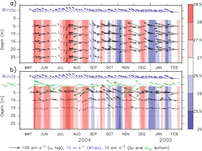
Fig. 3. Five-day-averaged time series of the 2°N, 140°W winds (blue vectors), temperature (color shading), and (a) currents (black vectors) and (b) currents relative to 20 m (black vectors) and surface geostrophic current relative to 20 m (green vectors). The vector scale for the currents, winds, and relative currents is shown at the bottom.
The time series of the 5-day-averaged measurements at 2°N, 140°W (Fig. 3a) show that, during the cool phase of the TIW, the upper ocean flow tends to be northward and, during the warm phase, the flow tends to be southward (Flament et al. 1996). The observed shears (Fig. 3b) also appear to be influenced by the passage of the fronts, although the pattern is not as distinct as for the current measurements. The sensitivity to wind and frontal variations, however, is clearly seen when the composite TIW is computed following the methodology described in section 3.
The anomalous southeastward currents during the warm phase and northwestward currents during the cool phase are seen in more detail in the TIW composite shown in Fig. 4a. Thermal wind shear is, by definition, parallel to the front, with cool water to the left and warm water to the right of the shear. The mean thermal wind shear composite is strongest and oriented to the southwest on the leading edge of the TIW cusp as the TIW transitions to its cool phase (Fig. 4c). At this stage of the wave, the southeasterly trade winds are most oblique to the front. During the subsequent cool phase, the mean thermal wind shear is somewhat westward. Then, during the transition to the warm phase of the TIW, on the trailing edge of the cusp, the thermal wind shear becomes northwestward. At this stage of the wave, the winds are nearly parallel to the front.
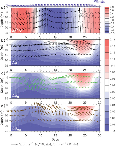
Fig. 4. Mean tropical instability wave composite (1 Nov 2004–28 Feb 2005) of (a) anomalous temperature (color), anomalous velocity (black vectors), and wind (blue vectors); (b) temperature relative to 28.3 m (color) and velocity relative to 20 m (black vectors); (c) as in (b) but for geostrophic currents relative to 20 m (green vectors); and (d) as in (b) but for ageostrophic currents relative to 20 m (brown vectors). The vector scale is shown at bottom.
During the warm phase, the southeasterly trades are more zonal and observed shears are nearly westward; while during the cool phase and the transition to the warm phase, observed shears are oriented to the northwest, roughly in the direction of the southeasterly trades (Fig. 4b). The small increase in the easterly trade winds prior to the transition to the TIW cool phase has been noted by several authors (e.g., Chelton et al. 2001). For most of the TIW cycle, however, the winds are steady.
On the basis of the classical Ekman model (4), one might expect that, if the winds are steady, the ageostrophic shears should be steady too. However, the ageostrophic shears have a strong TIW signal, with fluctuations of roughly ±4 cm s−1 over 15 m (Fig. 4d). In particular, the mean ageostrophic shear is largest and oriented northwestward during the transition to the cool phase when the geostrophic thermal wind is oriented southwestward, oblique to the wind. The ageostrophic shear also is relatively large and oriented in the direction of the wind during the transition to the warm phase when the wind blows along the front and the stratification is strong.
The observed currents relative to 20 m tend to be aligned with the wind as expected from the surface boundary condition (2b). Thus, in contrast to the large TIW swings in the geostrophic and ageostrophic shears, the observed currents relative to 20 m (Fig. 4b), like the winds, have a relatively steady orientation throughout most of the TIW. The magnitude of the shear, however is not steady; instead, its variation appears to be associated with changes in the stratification. The observed flow relative to 20 m (Fig. 4b) is weakest during the warm phase on day 5 when the stratification is weakest and has a local maximum when stratification is strongest: on day 15 during the cool phase and on day 24 during the transition to warm phase. Mixing and restratification likely affect the turbulent viscosity of the fluid and thus the shear that can be supported for a given stress. We note, though, that the maximum composite stratification is less than 0.07°C over 27.3 m, and that by most standards the upper 20 m would be considered always well-mixed throughout the TIW cycle.
In summary, as expected from the surface boundary condition (2b) with relatively steady wind stress, variations in the near-surface shear appear to be primarily due to variations in the turbulent viscosity as inferred from the stratification. Both geostrophic and ageostrophic components contribute strongly to the total shear with the geostrophic component determined by the orientation and strength of the front. The ageostrophic shear thus arises from the imbalance between the wind stress and the stress associated with the thermal wind shear. When the winds are nearly aligned with the front during the transition to the warm phase (on the trailing edge of the TIW cusp), the thermal wind shear is too weak to balance the wind stress, resulting in a near-surface residual ageostrophic shear in the direction of the wind. Likewise, the front, and thus the thermal wind shear, is strongest and most oblique to the southeasterly trade winds during the transition from the warm to cool phase (on the leading edge of the cusp). Consequently, a large northward ageostrophic shear must be combined with the thermal wind shear to satisfy the surface stress boundary condition (2b). The ageostrophic shear depends on the orientation and relative strength of the wind to the front rather than strictly upon the wind itself.
The influence of stratification, and by inference viscosity, on the shears can be isolated by considering the diurnal cycle since the wind and front have little diurnal variability. Figure 5 shows the diurnal composite of the wind, near-surface currents relative to 25 m, and temperature, computed over the 4.5-month period when all five current meters were functioning. The top 25 m is isothermal (or even slightly unstable) at nighttime and is weakly stratified during the afternoon. Because the diurnal cycle of the winds is very weak, diurnal variations in the shear must be due to the influence of mixing and stratification (Price et al. 1986; Lien et al. 1995): During the afternoon, the albeit weak [0.1°C (10 m)−1] stratification causes the wind-generated momentum to be trapped within the shallow mixed layer. The shear associated with the afternoon "diurnal" jet is roughly aligned with the wind, while below the jet the shear is more zonal. By 1600 local time, the diurnal jet has currents at 5 m that are more than 12 cm s−1 stronger than at 25 m. As the diurnal warm layer cools and thickens during the late afternoon–early evening, the anomalous wind current can be seen at ever greater depths.
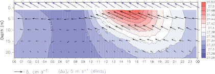
Fig. 5. Mean diurnal composite (24 May 2004–7 Oct 2004) of wind (blue vectors), temperature (color shading), and currents relative to 25 m (black vectors). The vector scale is shown at the bottom.
To better understand the mixing physics and viscosity properties associated with the diurnal cycle, a composite Richardson number is computed by dividing the composite buoyancy frequency (N2 = −g/ρ0 ∂ρ/∂z) by the composite squared shear (i.e., Ri = N2/|∂u/∂z|2). This method was found to be less noisy than computing the composite directly from the 20-min Ri time series. It should be noted that most Ri-based parameterizations of viscosity are not valid for unstable stratification in which Ri is negative. For example, in the commonly used Pacanowski and Philander (1981) parameterization, viscosity has a maximum value of 10.1 × 10⁻³ m2 s−1 for Ri = 0, while in the Peters et al. (1988) parameterization viscosity becomes unbound as Ri approaches zero. Since, Ri is slightly negative during nighttime (Fig. 6), indicating active convective mixing, nighttime turbulent viscosity is likely significantly larger than 10 × 10−3 m2 s−1. In contrast, between 1200 and 1400 local time, daytime warming causes stratification near 10 m to increase. The resulting Ri is larger than 0.25 and viscosity is thus expected to be smaller [roughly 2 × 10⁻³ m2 s−1 according to the Pacanowski and Philander (1981) and Peters et al. (1988) formulations]. At all other depths and times, Ri is less than 0.25, but positive, indicating that shear instability mixing is likely occurring. Interestingly, the critical Ri value of 0.25 appears to propagate downward with time, suggesting that as mixing transmits the wind-generated momentum and solar radiation warmed water to greater depths, shear is introduced, which causes the mixing to also be transmitted to greater depths, consistent with the model study of Danabasoglu et al. (2006). Averaged over the full diurnal cycle, the observed mean Ri increases with depth (Fig. 7), indicating that viscosity decays with depth, consistent with the assumption in our generalized Ekman model (7).
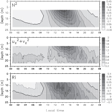
Fig. 6. Mean diurnal composite of (a) buoyancy frequency N2, (b) shear squared, and (c) Richardson number. The units in (a) and (b) are 10−4 s−1; Ri in (c) is nondimensional.
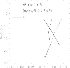
Fig. 7. Mean profiles of N2 (short dashed), shear squared (long dashed), and Ri (solid) averaged over the diurnal composite shown in Fig. 6.
The fundamental principle highlighted in this study is that the balance between the wind stress and the surface shear, expressed in the standard surface boundary condition (τ0 = ρ0ν ∂u/∂z), requires consideration of both the geostrophic and ageostrophic components of the shear. In horizontally homogenous regions, the near-surface geostrophic (thermal wind) shear is negligible and thus the surface shear that balances the wind stress is entirely ageostrophic, as in the balances of Ekman (1905) and Stommel (1960). In frontal regions, however, the geostrophic shear can be substantial, particularly in the tropics where the 1/f factor is large. When winds blow along a front, wind stress may be partially or entirely balanced by the geostrophic shear. As a consequence, the ageostrophic shear required to make the total shear balance the wind stress may be much smaller than expected.
Two models were introduced to describe the mean near-surface shear in the cold tongue front region at 2°N, 140°W: a frontal Ekman model (5) and a generalized Ekman model (7). Both models assume steady, linear flow. As with the classical Ekman model (4), the frontal Ekman model assumes that viscosity is vertically uniform, but differs from (4) by allowing a vertically uniform density front and, thus, a vertically uniform geostrophic shear. At the bottom of the frictional layer, the ageostrophic flow is assumed to be zero; while at the surface, the total (geostrophic and ageostrophic) shear is assumed to be proportional to the wind stress. The top boundary condition for the ageostrophic shear thus depends not only upon the wind stress, but also upon the strength and orientation of the front. The resulting solution for the ageostrophic shear is that of a classical Ekman model forced by the portion of the wind stress that is out of balance with the surface geostrophic shear.
At 2°N, 140°W, warm water lies to the north and west and the surface geostrophic shear was thus oriented to the southwest. With a viscosity estimated at 16 × 10−3 m2 s−1, the magnitude of the stress associated with surface thermal wind was comparable to that of the southeasterly trade wind stress. Consequently the westward component of the geostrophic shear nearly balanced the westward wind stress so that the effective surface stress that forced the ageostrophic shear was roughly northward. The resulting near-surface ageostrophic shear is primarily northward and rotates to the right (east) with depth, much like a classical Ekman spiral forced by a northward wind stress. When added to the geostrophic shear associated with the cold tongue front, the resulting total shear was more to the left (i.e., more westward) than the wind stress, as observed (Figs. 2a,c).
The generalized Ekman model is the vertical derivative of the steady, linear equations of motion (1), with shear written in terms of stress according to (2a). The model requires the prescribed viscosity to decay to zero at the level of no stress, but does not require the prescribed horizontal density gradient to be zero (as required by the classical Ekman model), nor be vertically uniform (as required by the frontal Ekman model). Furthermore, the generalized model is valid on the equator, while both the classical and frontal Ekman models are not.
For the generalized Ekman model at 2°N, 140°W (Fig. 2d), the front was assumed to be vertically uniform and viscosity was assumed to decay exponentially to a value of zero by twice the decay scale (set to 125 m, the top of the thermocline). When forced by the observed mean wind stress, the generalized Ekman model, like the frontal Ekman model, predicted currents relative to 25 m that were to the left of the mean wind stress, roughly in agreement with the observed currents relative to 25 m (Figs. 2a,d). Although the data clearly show that the classical Ekman model (4) is inappropriate for this region (Figs. 2a,b), the simulations from the frontal and generalized Ekman models are quite similar and both agree well with the observations. Indeed, with a layer depth of 250 m, similar to that used in the generalized model, and with viscosity and a buoyancy gradient similar to that used in the frontal model, the Bonjean and Lagerloef (2002) model also produced currents relative to 25 m that were to the left of the wind stress (not shown). These models differ primarily in their bottom boundary conditions and thus their differences would likely become more apparent with deeper data. The shallow observations studied here cannot definitively distinguish between these modified Ekman models.
A composite tropical instability wave illustrates the sensitivity of the ageostrophic shear to the orientation of the front relative to the winds (Fig. 4). Although winds were relatively steady throughout the cycle, the observed shear was less so, and the ageostrophic shear was not. During the transition from the cold phase to warm phase, when the front was aligned with the winds with warm water to the right, the near-surface ageostrophic shear was also aligned with the wind. During the transition from the warm phase to cold phase, when the front was oriented southwestward, oblique to the southeasterly winds, the near-surface shear had a large northward ageostrophic component that countered the southward component of the geostrophic thermal wind shear.
This is not the first study to recognize that in frontal regions the near-surface geostrophic shear contributes to the frictional stress. The shear equation derived by BL02 explicitly treats shear as a whole, rather than as composed of geostrophic and ageostrophic components. As shown by Garrett and Loder (1981), Thompson (2000), Flament and Armi (2000), Nagai et al. (2006), and others, the geostrophic contribution to the frictional stress produces an Ekman transport that is to the left of the geostrophic shear (i.e., toward the cold side of the front). Since this transport is maximum at the center of the front, it implies convergence and downwelling on the cold side of the front and divergence and upwelling on the warm side of the front. The wind stress thus tends to enhance this secondary circulation when the winds blow up a front, and tends to oppose it when the winds blow down a front, as is the case at 2°N, 140°W. Using a semigeostrophic model, Thompson (2000) showed that the resultant secondary circulation tends to spin down the front when the winds blow up a front, and tends to maintain the front when winds blow down the front.
The poleward currents observed in this study were substantially weaker than Johnson et al. (2001)'s mean poleward currents that were based upon nine years of shipboard ADCP sections between 95° and 170°W. A southwestward oriented front, such as observed at 2°N, 140°W, reduces the expected northward current in two ways: by causing the southward geostrophic current to be surface intensified and by causing a westward geostrophic frictional stress that tends to balance the westward wind stress. If these frontal effects do, in fact, cause a local minimum in the surface poleward flow near 2°N, 140°W, this may not be evident in the Johnson et al. (2001) shipboard ADCP section due to the considerable temporal, meridional, and zonal averaging done in that analysis. If this is the case, then the cold tongue front would likely be associated with a secondary circulation that had downwelling on the cold side of the front and upwelling on the warm side. With a single mooring, however, this deduction is speculative. Likewise, with only five current meters on a single mooring, we cannot directly measure the ageostrophic transport, nor its heat transport. We note however that, because the ageostrophic Ekman currents depend upon the orientation of the front, care must be taken in diagnosing the Ekman heat transport.
Viscosity is generally not known and must be parameterized. In our analysis we found that a value of 16 × 10−3 m2 s−1 produced shears in the Ekman models (Figs. 2b–d) with similar magnitude to the observed near-surface shear. The value is more than three times larger than the Santiago-Mandujano and Firing (1990) wind speed–based parameterization. However, those measurements were made during the 1982/83 El Niño, when the cold tongue front was absent or not well developed, the thermocline was anomalously deep, and the surface mixed layer conditions were quite different than normal (Cronin and Kessler 2002). We note also that the Peters et al. (1988) turbulence measurements at 0°, 140°W indicate that viscosity averaged from 23- to 49-m depth have nighttime values of approximately 10 × 10−3 m2 s−1 (see their Fig. 16). Nighttime convective mixing likely causes the viscosity values above 23 m to be significantly higher than this. Although our study has no current measurements below 25 m, the observed mean Richardson number within the upper 25 m increases with depth (Fig. 7), indicating that viscosity in all likelihood decays with depth.
The influence of even weak stratification on the magnitude of the near-surface shear could be seen both in the tropical instability wave and the diurnal cycle composites. As shallow stratification forms during the day, a diurnal jet develops. The afternoon (1600 local time) mean diurnal jet was ∼12 cm s−1 faster in the direction of the wind at 5 m than at 25 m, while nighttime mean shears were very weak (less than 4 cm s−1 over 20 m). Because the winds were relatively steady, these changes must be due to changes in the viscosity associated with nighttime mixing and daytime restratification. The composite analysis also showed that, as the diurnal warm layer cooled and thickened during the late afternoon–early evening, the wind-trapped momentum can be seen at ever greater depths. The resulting downward propagation of shear-induced mixing is evident in the diurnal composite of the Richardson number and is consistent with the model study of Danabasoglu et al. (2006).
Wijffels et al. (1994) showed that a diurnal jet can form even for stratification that by many criteria would be considered mixed, and that a slab layer was observed only when a stringent definition of the mixed layer was used. In our case, the mean afternoon stratification between 1 and 25 m was ∼0.18°C, which is considered weakly stratified by their criteria. At nighttime, when the mean stratification was near zero, shears were very weak and the layer was more slablike. Although the nighttime shear is near the instantaneous measurement error of the Sontek current meters, the ensemble mean is significant if the errors are random. Nighttime mixing is not 100% efficient at removing shears, in part because the eddy viscosity, while large, is not infinite. The overall mean stratification was extremely weak (0.07°C over 27.3 m) and met the Wijffels et al. slab layer criteria. Yet, while the mean meridional currents were vertically uniform, the zonal currents were sheared (Fig. 1). Mixing should act on the total shear, not simply on the meridional component. Therefore, the uniform poleward currents on their own cannot be interpreted as evidence of a slab layer.
Finally, it remains an open question as to how the diurnal cycles of stratification, shear, and mixing influence the observed Ekman spiral. On the one hand, since mixing is a one-way process and the inertial time scale at 2°N is much longer than a day, nighttime mixing could set the overall effective viscosity. In that case, the viscosity that determines the Ekman spiral would be larger and extend deeper than might be expected based upon the mean stratification. The Danabasoglu et al. (2006) downward propagation of shear-instability mixing beginning in the late afternoon provides another mechanism by which the influence of wind forcing is felt below near-surface stratification.
Alternatively, the observed strong diurnal jet (Figs. 4–6) suggests that the Ekman spiral at 2°N, 140°W may be dominated by the afternoon stratification. Aspects of stratified Ekman spirals have been observed in the midlatitudes by Price et al. (1987) and Chereskin (1995), near the equator by Santiago-Mandujano and Firing (1990), along 10°N in the Pacific by Wijffels et al. (1994), along 11°N in the Atlantic by Chereskin and Roemmich (1991), and in the Arabian Sea by Chereskin et al. (1997). None of these studies, however, were in strong frontal regions. Indeed, metrics used to identify a stratified Ekman layer may need to be reconsidered for frontal regions. Price and Sundermeyer (1999) argued that at mid and high latitudes, currents in a stratified Ekman spiral are more strongly surface intensified than if the spiral occurred fully within a well-mixed layer. That is, a stratified Ekman spiral at these latitudes is flatter with thinner, faster layers near the surface and slower, thicker layers in the lower portion of the spiral. At low latitudes, Price and Sundermeyer hypothesized that the diurnal stratification would have less importance. Because our deepest measurement was at 25 m, the lower portion of the spiral at 2°N was not observed here. Thus, our study is unable to differentiate between the contrasting effects on the Ekman spiral of momentum trapping by near-surface stratification and leakage of momentum into the deeper water through nighttime and late-afternoon mixing.
Acoustic Doppler current profilers have been used with great success to monitor vertical shear in oceanic currents. However, whether mounted on ships or moored at depth, these profiles have a "blind spot" near the surface, precisely where we expect the strongest response to wind forcing. The Johnson et al. (2001) compilation suggests that more than 50% of the meridional overturning cell's poleward transport across 2°N lies above 15 m. For downward-looking shipboard ADCPs, the depth of the first measurement bin is determined by the depth of the ship's hull and the blanking depth of the sensor; for upward-looking moored ADCPs, the top bin is determined by the depth of the ADCP and the angle of its beams (Gordon 1996). For most applications such profilers have been set up to monitor the current structure between 250 and 25 m, and the current profiles must generally be extrapolated to the surface for calculations of, for example, mixed layer velocity, integrated transport, transport divergence, and vertical velocity. Extrapolations in these cases are typically based upon some assumption of the shear within the top 25 m, either that it is zero (i.e., a slab layer) or that it is uniform and equivalent to the shear at ∼25–30-m depth.
Using a set of five current meters mounted at 5-m intervals between 5-m and 25-m depth on a test mooring in the cold tongue front at 2°N, 140°W, we show that the near-surface shear is highly sensitive to the vertical and horizontal temperature (i.e., density) distribution. In particular, the horizontal density gradient gives rise to a geostrophic (thermal wind) shear that affects the dynamics in (at least) two ways: through the surface boundary condition (2b), where it is part of the total shear and acts as a component of the effective stress forcing the ageostrophic shear, and as part of the interior shear that is added to that ageostrophic shear forced by the effective surface stress. At 2°N, 140°W, the SST front is oriented southwestward, with cool water to the south and east, while the trade winds are to the northwest. Thus, the mean zonal component of the thermal wind shear is westward, tending to balance the westward wind stress and, as a result, the ageostrophic shear required to balance the zonal wind stress is small. On the other hand, the meridional component of thermal wind shear is southward. A large northward ageostrophic surface shear is thus required to balance the northward wind stress. The net effect is that the observed Ekman-like ageostrophic spiral is shifted roughly 60° to the right of the expected classical Ekman spiral. At 2°N, 140°W this dynamic, combined with the southwestward thermal wind shear, was manifest in total (measured) near-surface shears that were oriented to the left of the wind stress. The near-surface shear is not a linear combination of the geostrophic thermal wind shear and shear associated with the classical Ekman spiral. We show, instead, that realistic ageostrophic currents with an Ekman-like spiral were reproduced when the Ekman equation was forced by the portion of the wind stress that is out of balance with the surface geostrophic shear. We refer to this as the "frontal Ekman" model. Alternatively, the shear equation can be written in terms of stress, with the requirement that at the depth of no stress the viscosity is zero. The resulting "generalized Ekman" model is valid both in frontal regions and on the equator. Both the frontal and generalized Ekman models produced near-surface currents relative to 25 m that were in qualitative agreement with those observed at 2°N, 140°W.
Considering that the Ekman (1905) model is over a hundred years old, it is somewhat surprising to the au-thors that its failure in frontal regions has not been thoroughly studied. This may be because the geostrophic shear depends upon 1/f and therefore decreases with latitude. That is, the surface thermal wind stress magnitude may be comparable to the wind stress only in frontal regions in the tropics. Another reason may be that near-surface shear measurements are very rare. The present study is based upon five current meters with thermistors in the top 25 m of a surface mooring at 2°N, 140°W. Although a single mooring in the frontal region at 2°N, 140°W was sufficient to see the influence of the front on the Ekman spiral, a more comprehensive observing strategy would be necessary to resolve the influence of the front on the vertical motion. Our results suggest that the front might have a narrow meridional-vertical (secondary) circulation cell that splits the tropical Pacific meridional overturning cell into two or three cells. This, however, cannot be resolved with the present data.
The authors thank the TAO project office and the PMEL Engineering Development Division for assistance with this project. In particular, the authors wish to thank Paul Freitag, Patricia Plimpton, Sonya Noor, Curren Fey, and David Zimmerman for their help processing the data and preparing the sensors. The authors also thank three anonymous reviewers and LuAnne Thompson, Lief Thomas, Eric D'Asaro, RenChieh Lien, Fabrice Bonjean, Renellys Perez, ChuanLi Jiang, and Andy Chiodi for illuminating discussions of this work. Support for this work was provided by the NOAA/Climate Programs Office and Office of Oceanic and Atmospheric Research.
Ando, K., and M. J. McPhaden, 1997: Variability of surface layer hydrography in the tropical Pacific Ocean. J. Geophys. Res., 102, 23 063–23 078.
Bloomfield, P., 1976: Fourier Decomposition of Time Series: An Introduction. Wiley, 258 pp.
Bonjean, F., and G. S. E. Lagerloef, 2002: Diagnostic model and analysis of the surface currents in the tropical Pacific Ocean. J. Phys. Oceanogr., 32, 2938–2954.
Bryden, H. L., and E. C. Brady, 1985: Diagnostic model of the three-dimensional circulation in the upper equatorial Pacific Ocean. J. Phys. Oceanogr., 15, 1255–1273.
Chelton, D. B., and Coauthors, 2001: Observations of coupling between surface wind stress and sea surface temperature in the eastern tropical Pacific. J. Climate, 14, 1479–1498.
Chereskin, T. K., 1995: Direct evidence for an Ekman balance in the California Current. J. Geophys. Res., 100, 18 261–18 269.
Chereskin, T. K., and D. Roemmich, 1991: A comparison of measured and wind-derived Ekman transport at 11°N in the Atlantic Ocean. J. Phys. Oceanogr., 21, 869–878.
Chereskin, T. K., W. D. Wilson, H. L. Bryden, A. Ffield, and J. Morrison, 1997: Observations of the Ekman balance at 8°30'N in the Arabian Sea during the 1995 southwest monsoon. Geophys. Res. Lett., 24, 2541–2544.
Cronin, M. F., and W. S. Kessler, 2002: Seasonal and interannual modulation of mixed layer variability at 0°, 110°W. Deep-Sea Res. I, 49, 1–17.
Cronin, M. F., N. Bond, C. Fairall, J. Hare, M. J. McPhaden, and R. A. Weller, 2002: Enhanced oceanic and atmospheric monitoring underway in eastern Pacific. Eos, Trans. Amer. Geophys. Union, 83, 205, doi:10.1029/2002EO000137. 210–211.
Danabasoglu, G., W. G. Large, J. J. Tribbia, P. R. Gent, B. P. Briegleb, and J. C. McWilliams, 2006: Diurnal coupling in the tropical oceans of CCSM3. J. Climate, 19, 2347–2365.
Ekman, V. W., 1905: On the influence of the earth's rotation on ocean-currents. Ark. Mat. Astron. Fys., 2, 1–52.
Fairall, C. F., E. F. Bradley, J. E. Hare, A. A. Grachev, and J. B. Edson, 2003: Bulk parameterization of air–sea fluxes: Updates and verification for the COARE algorithm. J. Climate, 16, 571–591.
Flament, P., and L. Armi, 2000: The shear, convergence, and thermohaline structure of a front. J. Phys. Oceanogr., 30, 51–66.
Flament, P., S. Kennan, R. Knox, P. Niiler, and R. Bernstein, 1996: The three-dimensional structure of a tropical instability wave. Nature, 383, 610–613.
Freitag, H. P., Y. Feng, L. J. Mangum, M. J. McPhaden, J. Neander, and L. D. Stratton, 1994: Calibration procedures and instrumental accuracy estimates of TAO temperature, relative humidity and radiation measurements. Tech. Memo. ERL PMEL-104 (PB95-174827), NOAA, Pacific Marine Environmental Laboratory, Seattle, WA, 32 pp.
Freitag, P., M. McPhaden, C. Meinig, and P. Plimpton, 2003: Mooring motion bias of point Doppler current meter measurements. Proc. IEEE Seventh Working Conf. on Current Measurement Technology, San Diego, CA, IEEE, 155–160.
Garrett, C. J. R., and J. W. Loder, 1981: Dynamical aspects of shallow sea fronts. Philos. Trans. Roy. Soc. London, 302A (1472), 563–581.
Gordon, R. L., 1996: Acoustic Doppler Current Profilers, Principles of Operation: A Practical Primer. R. D. Instruments, 51 pp. [Available from R. D. Instruments, 9855 Businesspark Ave., San Diego, CA 92131.]
Halpern, D., and H. P. Freitag, 1987: Vertical motion in the upper ocean of the equatorial Pacific. Oceanol. Acta, (Special Vol.), 19–26.
Johnson, G. C., M. J. McPhaden, and E. Firing, 2001: Equatorial Pacific Ocean horizontal velocity, divergence, and upwelling. J. Phys. Oceanogr., 31, 839–849.
Kug, J.-S., I.-S. Kang, and S.I. An, 2003: Symmetric and anti-symmetric mass exchanges between the equatorial and off-equatorial Pacific associated with ENSO. J. Geophys. Res., 108, 3284, doi:10.1029/2002JC001671.
Lien, R.-C., D. R. Caldwell, M. C. Gregg, and J. N. Moum, 1995: Turbulence variability at the equator in the central Pacific at the beginning of the 1991–1993 El Niño. J. Geophys. Res., 100, 6881–6898.
McPhaden, M. J., M. F. Cronin, and D. C. McClurg, 2008: Surface mixed layer temperature balance on seasonal time scales in the eastern tropical Pacific. J. Climate, 21, 3240–3260.
Meinen, C. S., M. J. McPhaden, and G. C. Johnson, 2001: Vertical velocities and transports in the equatorial Pacific Ocean during 1993–99. J. Phys. Oceanogr., 31, 3230–3248.
Nagai, T., A. Tandon, and D. L. Rudnick, 2006: Two-dimensional ageostrophic secondary circulation at ocean fronts due to vertical mixing and large-scale deformation. J. Geophys. Res., 111, C090938, doi:10.1029/2005JC002964.
Pacanowski, R. G., and S. G. H. Philander, 1981: Parameterization of vertical mixing in numerical models of the tropical ocean. J. Phys. Oceanogr., 11, 1443–1451.
Peters, H., M. C. Gregg, and J. M. Toole, 1988: On the parameterization of equatorial turbulence. J. Geophys. Res., 93, 1199–1218.
Peters, H., R. A. Weller, and R. Pinkel, 1986: Diurnal cycling: Observations and models of the upper ocean response to diurnal heating, cooling and wind mixing. J. Geophys. Res., 91, 8411–8427.
Peters, H., R. A. Weller, and R. R. Schudlich, 1987: Wind-driven ocean currents and Ekman transport. Science, 238, 1534–1538.
Price, J. F., and M. A. Sundermeyer, 1999: Stratified Ekman layers. J. Geophys. Res., 104, 20 467–20 494.
Santiago-Mandujano, F., and E. Firing, 1990: Mixed-layer shear generated by wind stress in the central equatorial Pacific. J. Phys. Oceanogr., 20, 1576–1582.
Schneider, N., and P. Müller, 1994: Sensitivity of the surface equatorial ocean to the parameterization of vertical mixing. J. Phys. Oceanogr., 24, 1623–1640.
Smyth, W. D., D. Hebert, and J. N. Moum, 1996: Local ocean response to a multiphase westerly wind burst. 1. Dynamic response. J. Geophys. Res., 101, 22 495–22 512.
Stommel, H., 1960: Winddrift near the equator. Deep-Sea Res., 6, 298–302.
Thompson, L., 2000: Ekman layers and two-dimensional frontogenesis in the upper ocean. J. Geophys. Res., 105 (C3), 6437–6451.
Weisberg, R. H., and L. Qiao, 2000: Equatorial upwelling in the central Pacific estimated from moored velocity profiler. J. Phys. Oceanogr., 30, 105–124.
Wijffels, S., E. Firing, and H. Bryden, 1994: Direct observations of the Ekman balance at 10°N in the Pacific. J. Phys. Oceanogr., 24, 1666–1679.
Willett, C. S., R. R. Leben, and M. F. Lavín, 2006: Eddies and tropical instability waves in the eastern tropical Pacific: A review. Prog. Oceanogr., 69, 218–238.
Wyrtki, K., 1981: An estimate of equatorial upwelling in the Pacific. J. Phys. Oceanogr., 11, 1205–1214.
Go to Abstract
Go to Gallery of Figures
Go to References
Return to Outstanding Publications Page
Return to PMEL Publications Page
Return to PMEL Home Page