The study describes the development, testing and applications of site-specific tsunami inundation models (forecast models) for use in NOAA's tsunami forecast and warning system. The model development process includes sensitivity studies of tsunami wave characteristics in the nearshore and inundation, for a range of model grid setups, resolutions and parameters. To demonstrate the process, four forecast models in Hawaii, at Hilo, Kahului, Honolulu, and Nawiliwili are described. The models were validated with fourteen historical tsunamis and compared with numerical results from reference inundation models of higher resolution. The accuracy of the modeled maximum wave height is greater than 80% when the observation is greater than 0.5 m; when the observation is below 0.5 m the error is less than 0.3 m. The error of the modeled arrival time of the first peak is within 3% of the travel time. The developed forecast models were further applied to hazard assessment from simulated magnitude 7.5, 8.2, 8.7 and 9.3 tsunamis based on subduction zone earthquakes in the Pacific. The tsunami hazard assessment study indicates that use of a seismic magnitude alone for a tsunami source assessment is inadequate to achieve such accuracy for tsunami amplitude forecasts. The forecast models apply local bathymetric and topographic information, and utilize dynamic boundary conditions from the tsunami source function database, to provide site- and event-specific coastal predictions. Only by combining a Deep-ocean Assessment and Reporting of Tsunami-constrained tsunami magnitude with site-specific high-resolution models can the forecasts completely cover the evolution of earthquake-generated tsunami waves: generation, deep ocean propagation, and coastal inundation. Wavelet analysis of the tsunami waves suggests the coastal tsunami frequency responses at different sites are dominated by the local bathymetry, yet they can be partially related to the locations of the tsunami sources. The study also demonstrates the nonlinearity between offshore and nearshore maximum wave amplitudes.
The tragedy of the 2004 Indian Ocean tsunami made obvious the vulnerability of coastal populations to this deadly natural disaster and illustrated the need for effective forecasting. In the aftermath of the tsunami, the acceleration of development and implementation of more advanced tsunami forecast systems worldwide has become a major priority in the scientific and disaster management communities [Titov, 2009; Lautenbacher, 2005; Synolakis et al., 2005; Bernard et al., 2006; Geist et al., 2006; Synolakis and Bernard, 2006]. New forecast systems are being developed and implemented in many coastal nations. Major efforts are underway in the U.S, Japan, Australia, Indian and Indonesia [Titov, 2009; Kuwayama, 2007; Greenslade et al., 2007; Nayak and Kumar, 2008; Rudloff et al., 2008; Sobolev et al., 2006]. The U.S. system applies a combination of seismic and direct tsunami wave measurements with real-time inundation modeling for coastal predictions. Other systems are based primarily on indirect tsunami measurements (e.g., seismic and GPS shield data) and precomputed modeling.
After the 2004 Indian Ocean tsunami, the U.S. expanded the role of the National Tsunami Hazard Mitigation Program to implement the recommendations of the National Science and Technology Council [2005] to enhance tsunami forecast and warning capabilities along the U.S. coastlines. Toward these goals, the NOAA Center for Tsunami Research at NOAA's Pacific Marine Environmental Laboratory is developing a tsunami forecast system for NOAA's Tsunami Warning Centers [Titov et al., 2005; Titov, 2009]. The forecast system combines real-time deep ocean tsunami measurements from Deep-ocean Assessment and Reporting of Tsunami (DART) buoys [González et al., 2005; Bernard et al., 2006; Bernard and Titov, 2007] with the Method of Splitting Tsunami (MOST) model, a suite of finite difference numerical codes based on nonlinear long wave approximation [Titov and Synolakis, 1998; Titov and González, 1997; Synolakis et al., 2008] to produce real-time forecasts of tsunami arrival time, heights, periods and inundation. To achieve accurate and detailed forecast of tsunami impact for specific sites, high-resolution tsunami forecast models are being developed for U.S. coastal communities at risk. The resolution of these models has to be high enough to resolve the dynamics of a tsunami inside a particular harbor, including influences of major harbor structures such as breakwaters. These models have been integrated as crucial components into the forecast system.
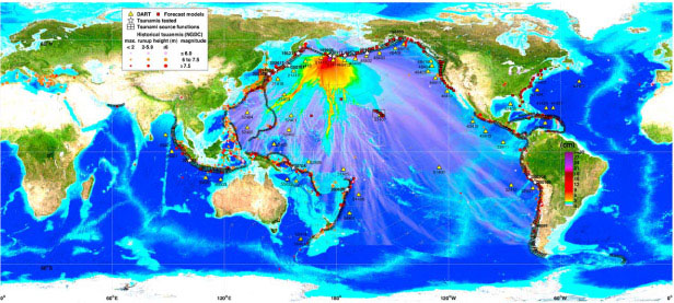
Presently, a system of 48 DART buoys (39 U.S., 1 Chilean, 6 Australian, 1 Thailand, and 1 Indonesia owned) is monitoring tsunami activity in the Pacific, Indian and Atlantic Oceans (Figure 1). The precomputed tsunami source function database currently contains 1691 scenarios to cover global tsunami sources, and the forecast models are now set up for 43 U.S. coastal communities. The fully implemented system will use real-time data from the DART network to provide high-resolution tsunami forecasts for at least 75 communities in the U.S. by 2013 [Titov, 2009]. Since its first testing in the 17 November 2003 Rat Islands tsunami, the forecast system has produced experimental real-time forecasts for 12 tsunamis in the Pacific and Indian oceans [Titov et al., 2005; Wei et al., 2008; Titov, 2009]. The forecast methodology has also been tested with the data from nine additional events that produced deep ocean data [Titov et al., 2005; Tang et al., 2008a]. In the study, we test fourteen tsunamis as summarized in Table 1 for model validation and forecast accuracy.
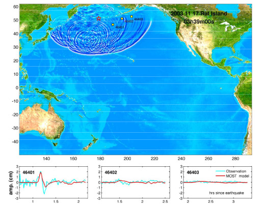
Fig. 1. Overview of the tsunami forecast system. Components of the system include DART systems (yellow triangles), precomputed tsunami source function database (black rectangles), and high-resolution forecast models (solid red squares). Colors show computed maximum tsunami amplitudes of the offshore forecast in cm using the 17 November 2003 Rat Islands tsunami as an example. Black contour lines indicate tsunami travel times in hours. Solid circles are historical tsunamis [National Geophysical Data Center, 2007].
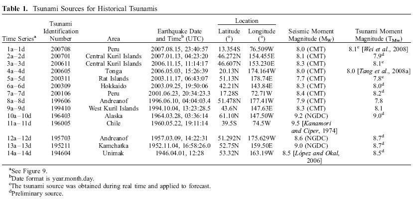
Table 1. Tsunami sources for historical tsunamis.
The three main components of the forecast system, the DART observing network, tsunami source function databases and the forecast models, reflect the three main stages of the evolution of tsunami waves: generation, deep ocean propagation, and coastal inundation. This study focuses on the last stage to provide the final products during a real-time tsunami forecast. Here we present an overview of the research toward development, validation and applications of the high-resolution forecast models by using sites in Hawaii as examples. Secondary objectives are to investigate local frequency responses to tsunamis by wavelet analysis; and the non-linearity between the offshore and nearshore wave heights.
Section 2 of this article introduces NOAA's tsunami forecast methodology and demonstrates forecast model setups for Hawaii. Section 3 describes the development and testing of the forecast inundation models. The development process includes creation of bathymetric and topographic data sets, model sensitivity studies, model validation and error estimation, and testing for model robustness and stability. Procedures for future model development are also suggested. Section 4 presents a tsunami hazard assessment study utilizing the validated forecast models and comparisons of modeled offshore and nearshore wave heights. Summary and conclusions are provided in section 5.
NOAA's real-time tsunami forecasting scheme is a process that comprises of two steps: (1) construction of a tsunami source via inversion of deep ocean DART observations with precomputed tsunami source functions and (2) coastal predictions by running high-resolution forecast models in real time [Titov et al., 1999, 2005].
In the context of this paper, a tsunami source is a sea surface deformation that generates a series of modeled long waves reproducing observed tsunami wave characteristics, including arrival time, height and period in deep ocean. Reconstructing a tsunami source does not necessarily require knowing the details of the earthquake focal mechanism [Wei et al., 2008; Tang et al., 2008a]. Wave dynamics of tsunami propagation in deep ocean is assumed to be linear [Liu, 2009]. Thus a tsunami source can be effectively constructed based on the best fit to given deep ocean tsunami measurements from a linear combination of precomputed tsunami source functions.
The sea surface deformation is computed using an elastic deformation model [Gusiakov, 1978; Okada, 1985]. This deformation directly links the tsunami source functions with the earthquake fault parameters and magnitudes. The deformation model assumes that an earthquake can be modeled as the rupture of a single rectangular fault plane that is characterized by parameters describing the location, orientation and rupture direction of the plane. Titov et al. [1999, 2001] conducted sensitivity studies on far-field deep water tsunamis to different parameters of the deformation model, including length of the rupture plane, the width of the plane, the depth of the source, dip angle, strike angle and the average slip amount. The results showed source magnitude and location essentially define far-field tsunami signals for a wide range of subduction zone earthquakes. Other parameters have secondary influence and can be predefined during forecast. Based on these results, tsunami source function databases for Pacific, Atlantic, and Indian Oceans have been built using predefined source parameters with length 100 km, width 50 km, slip 1 m, rake 90 and rigidity 4.5 × 10¹⁰ N/m2. Other parameters are location specific; details of the databases are described by Gica et al. [2008]. Each tsunami source function (TSF) is equivalent to a tsunami from a typical Mw = 7.5 earthquake with defined source parameters. Figure 1 shows the locations of tsunami source functions in the databases.
Several real-time data sources, including seismic data, coastal tide gauge and deep ocean data have been used for tsunami warning and forecast [Satake et al., 2008; Whitmore, 2003; Titov, 2009]. NOAA's strategy for the real-time forecasting is to use deep ocean measurements at DART buoys as the primary data source due to several key features. (1) The buoys provide a direct measure of tsunami waves, unlike seismic data, which are an indirect measure of tsunamis. (2) The deep ocean tsunami measurements are in general the earliest tsunami information available, since tsunamis propagate much faster in deep ocean than in shallow coastal area where coastal tide gauges are used for tsunami measurements. (3) Compared to coastal tide gauges, DART data with a high signal-to-noise ratio can be obtained without interference from harbor and local shelf effects. (4) The linear process of tsunamis in deep ocean allows application of efficient inversion schemes.
Time series of tsunami observations in deep ocean can be decomposed into a linear combination of a set of tsunami source functions in the time domain by a linear least squares method. We call coefficients obtained through this inversion process tsunami source coefficients. The magnitude computed from the sum of the moment of TSFs multiplied by the corresponding coefficients is referred as the tsunami moment magnitude (TMw), to distinguish from the seismic moment magnitude Mw, which is the magnitude of the associated earthquake source. While the seismic and tsunami sources are in general not the same, this approach provides a link between the seismically derived earthquake magnitude and the tsunami observation-derived tsunami magnitude. Under certain circumstances, Mw and TMw can be equal if the initial sea surface deformation of the DART-constrained tsunami source (linear combination of TSFs) would be the same as the surface deformation due to the seismically constrained fault model (usually a linear combination of finite faults). However, in most cases, they will be different due to factors ranging from different model assumptions defining these two magnitudes to the different physical processes that are recorded at seismometers and at tsunameters. While the numerical difference is usually small (partially due to the logarithmic scale of the magnitudes) in some rare cases it can be substantial. Though a thorough discussion about the relationship between the two magnitudes is out of the scope of this paper, it will be presented in forthcoming studies.
During real-time tsunami forecast, seismic waves propagate much faster than tsunami waves so the initial seismic magnitude can be estimated before the DART measurements are available. Since time is of essence, the initial tsunami forecast is based on the seismic magnitude only. The TMw will update the forecast when it is available via DART inversion using the TSF database. As will be shown in our examples, TMw appears to be a robust measure of the tsunami impact. So we focus our forecast analysis on defining TMw.
The database can provide offshore forecast of tsunami amplitudes and all other wave parameters immediately once the inversion is complete. The tsunami source, which combines real-time tsunami measurements with tsunami source functions, provides an accurate offshore tsunami scenario without additional time-consuming model runs.
High-resolution forecast models are designed for the final stage of the evolution of tsunami waves: coastal inundation. The DART-constrained tsunami source, corresponding offshore scenario from the TSF database, and site-specific forecast models cover the entire evolution, providing a complete tsunami forecast capability.
Once the DART-constrained tsunami source is obtained (as a linear combination of TSFs), the precomputed time series of offshore wave height and depth-averaged velocity from the model propagation scenario are applied as the dynamic boundary conditions for the forecast models. This saves the simulation time of basin wide tsunami propagation. Tsunami inundation is a highly nonlinear process, therefore a linear combination would not, in general, provide accurate solutions. A high-resolution model is also required to resolve shorter tsunami wavelengths nearshore with accurate bathymetric/topographic data. The forecast models are constructed with the Method of Splitting Tsunami (MOST) model, a finite difference tsunami inundation model based on nonlinear shallow water wave equations [Titov and González, 1997]. Each forecast model contains three telescoping computational grids with increasing resolution, covering regional, intermediate and nearshore areas. Runup and inundation are computed at the coastline. The highest resolution grid includes the population center and tide stations for forecast verification. The grids are derived from the best available bathymetric/topographic data at the time of development, and will be updated as new survey data become available. Figure 2 shows the forecast model setup for several tsunami forecast models in Hawaii, detailing the telescoping grids used. (1) One regional grid of 2 arc min (∼3600 m) resolution covers the main Hawaiian Islands (Figure 2a). (2) Then the Hawaiian Islands are divided into four intermediate grids of 12 to 18 arc sec (∼360–540 m) for four natural geographic areas: Ni'ihau, Ka'ula Rock, and Kauai (Kauai complex) (Figure 2b); Oahu (Figure 2c); Molokai, Maui, Lanai, and Kaho'olawe (the Maui Complex) (Figure 2d); and Hawaii (Figure 2e). (3) Each intermediate grid contains 2 arc sec (∼60 m) nearshore grids (Figures 2f–2i).
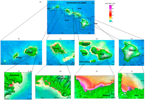
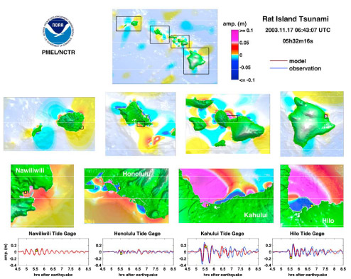
Fig. 2. Forecast model setups in Hawaii: (a) 2 arc min (∼3600 m) regional, (b–e) 12–18 arc sec (∼360–540 m) intermediate, and (f–i) 2 arc sec (∼60 m) nearshore grids for Nawiliwili, Honolulu, Kahului, and Hilo. Filled colors show the maximum tsunami amplitude in cm computed by the forecast models for the 17 November 2003 Rat Islands tsunami. Red dots, coastal tide stations; red crosses, offshore locations.
The forecast models are optimized for speed and accuracy. By reducing the computational areas and grid resolutions, each model is optimized to provide 4 hour event forecasting results in minutes of computational time using one single processor, while still providing good accuracy for forecasting. To ensure forecast accuracy at every step of the process, the model outputs are validated with historical tsunami records and compared to numerical results from a reference inundation model with higher resolutions and larger computational domains. Figure 3 shows the telescoping grids for the Kahului reference inundation model with 36, 6 and 1/3 arc sec (∼1080, 180 and 10 m) grid resolutions. In order to provide warning guidance for long duration during a tsunami event, each forecast model has been tested to output up to 24 hour simulation since tsunami generation.
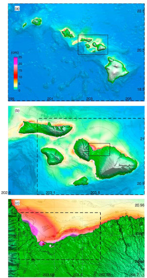
Fig. 3. Grid setup of the Kahului reference inundation model. The spatial resolutions are (a) 36 arc sec (∼1080 m), (b) 6 arc sec (∼180 m), and (c) 1/3 arc sec (∼10 m), respectively. Filled colors show the maximum amplitude in cm computed by the model for the 17 November 2003 Rat Islands tsunami. Solid lines, boundaries of the telescoping grids of the model; dashed lines, grid boundaries of the Kahului forecast model as in Figures 2a, 2d, and 2h.
Two types of gridded digital elevation models (DEMs) were developed for each study area; a DEM at medium resolution of 6 arc sec (∼180 m) for wave transformation from the open ocean to coastal areas; and a high resolution 1/3 arc sec (∼10 m) DEM for modeling of wave runup and inundation onto dry land. The grids for the forecast models and corresponding reference inundation model used by MOST model were sampled from these two DEMs.
The DEMs were compiled from several data sources. For example, Figure 4 is an overview of the spatial extents of each data source incorporated into the medium-resolution and the high-resolution DEMs for Kahului. Table 2 is an overview of the data sources used; in general, the data sources listed first superseded data sources listed later in the area where they overlapped. All selected input data sets were converted to the mean high water (MHW) vertical datum, as necessary. Horizontal positions were reprojected, where necessary, to the WGS84 horizontal geodetic datum. Details are given by Tang et al. [2008b].
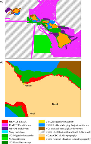
Fig. 4. Bathymetric and topographic data source overview. (a) Hawaiian Islands with 6 arc sec (∼180 m) resolution and (b) central Maui with 1/3 arc sec (∼10 m) resolution.
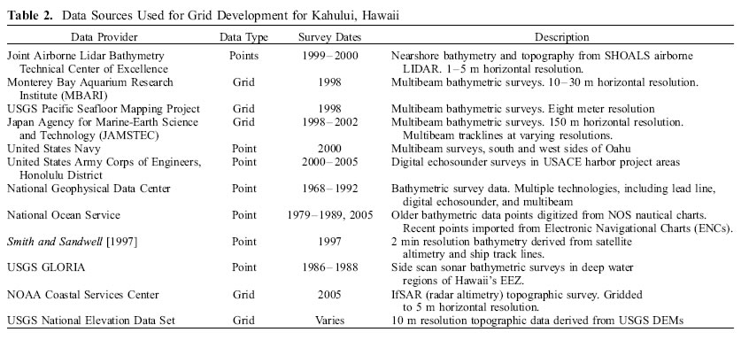
Table 2. Data sources used for grid development for Kahului, Hawaii.
How sensitive are the model outputs, including time series and inundation, to changes in the grid resolution, computational domains, accuracy of bathymetry/topography and other parameters? This issue is central to model development, because even with a correct tsunami source and a well-validated tsunami inundation numerical model, inappropriate model setup or inaccurate bathymetry/topography can produce poor or incorrect results.
Two case studies, at Kahului and Honolulu, were examined to evaluate the impact of model grid extent and resolution on the modeling results. For each tsunami, an identical tsunami source was applied to different model setups.
Figure 5a and Table 3 show how the changes of grid setup affect the model accuracy and speed at Kahului for the May 2006 Tonga tsunami. The grids for setups 1, 2 and 3 in Table 3, were derived from the same DEMs developed in 2005. Setups 1 and 2 are the first and revised Kahului forecast model. Setup 3 was the first Kahului reference inundation model. Prior to the 2006 Tonga tsunami, the forecast model setup 1 was tested with six past tsunamis, including the 2003 Rat Island, 2003 Hokkaido, 1996 Andreanof, 1994 Kuril Islands, 1964 Alaska and 1957 Andreanof tsunamis. Setup 1 produced good comparisons to these observations at Kahului tide station. The May 2006 Tonga event provided the first empirical test of the model with a wave propagating from the southwest. The incoming waves traveled through the shallow channels among the Maui Complex and exposed substantial deficiencies in the resolution and computational domain in the intermediate grid in setup 1. This illustrates the importance of testing tsunamis with all potential directionalities, especially for the Hawaiian Islands, which are in the middle of the Pacific Ocean. In 2007, nearshore bathymetric/topographic SHOALs airborne LIDAR with 1–5 m horizontal resolution from the Joint Airborne Lidar Bathymetry Technical Center of Expertise became available for Maui. Then the DEMs were updated and Kahului forecast and reference models were also redeveloped using the newest data source. More details on the updated models can be found at Tang et al. [2008b].
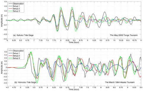
Fig. 5. Tsunami time series computed from different model setups at (a) Kahului tide gauge for the May 2006 Tonga tsunami and (b) Honolulu tide gauge for the March 1964 Alaska tsunami.
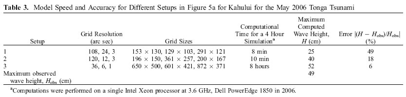
Table 3. Model speed and accuracy for different setups in Figure 5a for Kahului for the May 2006 Tonga Tsunami.
In Figure 5b, at Honolulu for the 1964 Alaska tsunami, grid setup 2, with a higher resolution, shows better comparison of wave height and phase for the later waves than those of setup 1. While model run time for a four hour simulation is less than ten minutes for setups 1 (120, 24, and 2 arc sec) and 2 (120, 18, and 2 arc sec), run time for the high-resolution setup 3 (36, 6 and 1/3 arc sec) is 64 hours. Finer resolution better resolves the individual structures of Honolulu harbor.
Tsunami forecast models for use in real-time operation need to balance between speed and accuracy. The models must complete within acceptable time limits, while using the highest resolution and largest computational domains possible. Currently, each forecast model is set up to run on a single processor in minutes. With the potential use of supercomputers in the future, the forecast speed can be further improved.
Accurate simulation of tsunami runup and inundation requires high quality runup and inundation data, high-resolution bathymetry and topography data in the runup area and good tsunami source parameters. Titov et al. [2005] have shown that, under these conditions, the MOST modeled runup and inundation agree quite well with survey data on Okushiri Island of the 12 July 1993 Hokkaido-Nansei-Oki Mw = 7.8 earthquake. At present, one major difficulty in inundation forecasting is a lack of high quality inundation/ runup measurements to verify the accuracy of topography and to calibrate the friction coefficient.
Topography/bathymetry compiled with incorrectly aligned datum or from different data sources can produce different inundation results. Figures 6a and 6b show the inundation computed from two sets of grids with the same 2 arc sec (∼60 m) resolution for the nearshore grids of Hilo forecast model for the 1946 Unimak tsunami. Grid 2 correctly reproduced the inundation limit as the measurements (Figure 6c), while no inundation was produced in grid 1 (Figure 6a). The topographic 0, 2, 5 and 10 m contours are quite different between these two grids. Developed in 2006 for the Hilo forecast model, all data sources for Grid 2 were converted to WGS 84 horizontal geodetic datum and mean high water vertical datum, when necessary. The data source for grid 1 was digitized and interpolated from the United States Geological Survey (USGS) maps.
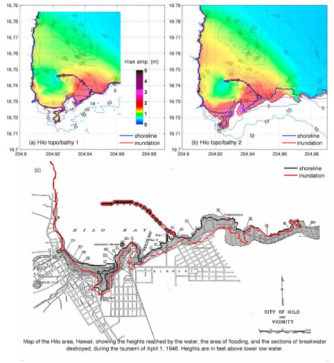
Fig. 6. (a and b) Maximum water elevations at Hilo computed from two sets of topographic and bathymetric grids for the April 1946 Unimak tsunami. (c) Comparison between computed inundation in Figure 6b and survey data from Shepard et al. [1950].
Figures 7a and 7b show how two topographic data sources produced different inundation results along the coastline from Ewa Beach to the Pearl Harbor entrance by a simulated TMw 9.3 tsunami from Solomon subduction zone near Santa Cruz Islands. Both nearshore grids have 1/3 arc sec (10 m) resolution. Recent high-resolution topographic LIDAR from the NOAA Coastal Services Center was applied in grid 2, which was developed for a tsunami hazard assessment study for Pearl Harbor [Tang et al., 2006]. The topographic data for grid 1 was derived from USGS 7.5 min DEM based on 30 m data spacing. The major 2, 5 and 10 m contours agree reasonably well for these two data sets. However, the topographic LIDAR data show a long narrow dune with an elevation around 2 m along Ewa Beach, which is absent in the USGS DEM. This explains the difference in inundation seen in Figure 7. Coastline with long narrow dunes is quite a common feature on the Hawaiian Islands. Attention must be paid to such features during grid development.
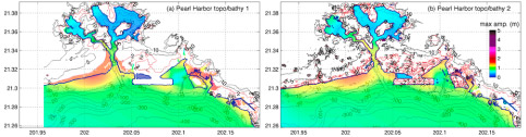
Fig. 7. Inundations at Pearl Harbor computed from two sets of topographic data sources used for a simulated TMw 9.3 tsunami. Topography was derived from (a) USGS DEM and (b) CSC LIDAR data. Color represents the maximum water elevation in m.
A smaller Manning coefficient can produce greater inundation over flat areas in some cases. However, the model can become unstable with a small Manning coefficient for certain large tsunami waves. Because of the model's sensitivity to the Manning coefficient, inundation extents may be subject to uncertainty in low-lying flat areas near the coast. The computed time series at a tide gauge location is generally less sensitive to the Manning coefficient setting. Figure 8 compares the inundation computed by the Kahului forecast model using different friction coefficients for two scenarios, (1) the April 1946 Unimak tsunami and (2) a simulated TMw 9.3 tsunami from Kamchatka. In Figure 8a, three different Manning coefficients, n = 0.01, 0.025 and 0.032, generate similar inundation lines for most of the coastline where the slope is relatively steep. However, the coefficient of 0.01 produces greater inundation in several flat areas such as the area southeast of Kahului Harbor. Figure 8b compares the inundation computed with n = 0.025 and 0.032 for the TMw 9.3 Kamchatka scenario. Though there are some minor differences at several locations, the inundation limit agrees well for this test case.
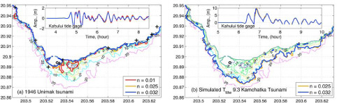
Fig. 8. Sensitivity of inundation and time series of tsunami amplitudes computed by the Kahului forecast model to Manning coefficients for (a) the April 1946 Unimak tsunami and (b) a simulated TMw 9.3 Kamchatka tsunami. Dots, Kahului tide gauge; crosses, Tsunami runup record from Pararas-Carayannis [1969].
The four forecast models in Hawaii and their corresponding higher resolution reference inundation models were tested with the fourteen historical tsunamis summarized in Table 1. Tide gauge data of the recent tsunamis, No.1 to 9, were from the NOAA National Water Level Observation Network (NWLON) [Allen et al., 2008], while others were digitized from Shepard et al. [1950], Zerbe [1953], Salsman [1959], Berkman and Symons [1964], and Spaeth and Berkman [1967]. The observations were filtered by a low-pass Butterworth filter with a cut-off of 60 or 120 min, to isolate lower-frequency components (including tide), which were then substracted from the raw data. In this section, we validate and evaluate the model performance through comparison of tsunami amplitude time series, period/frequency components via wavelet-derived spectra, and error estimation.
Figure 9 summarizes observed and modeled tsunami time series by the four forecast models at (1) Nawiliwili, (2) Honolulu, (3) Kahului, and (4) Hilo tide stations. When no observation is available, results from the forecast models were then compared with those computed by the higher resolution reference inundation models to ensure numerical consistency. The complete comparisons for each reference inundation model are documented in a technical report for each forecast site [Tang et al., 2008b, 2009].
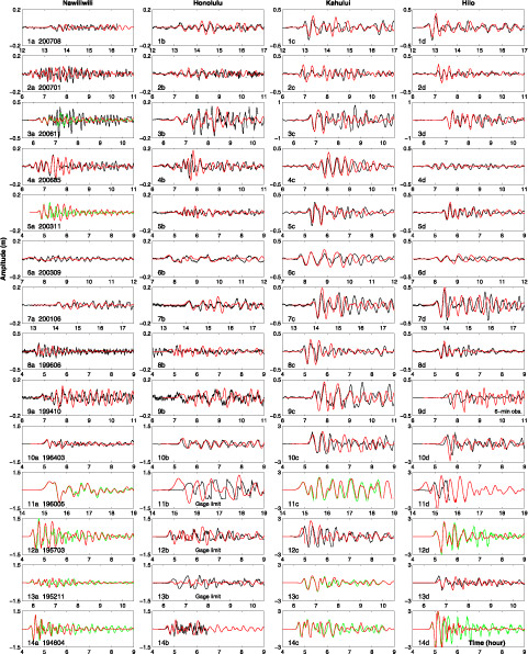
Fig. 9. Modeled and observed tsunami time series at Nawiliwili, Honolulu, Kahului, and Hilo tide stations for fourteen tsunamis. When no observation is available, results from the forecast models are compared with those from the reference inundation models. Black lines, observations; red lines, forecast models; green lines, reference inundation models. A 12 min adjustment was applied to the model time series 1a–1d for the August 2007 Peru tsunami.
Several recent tsunami events with a variety of geographic locations and source dynamics have provided rigorous tests of the forecast system. The most recent tested event is the 15 August 2007 Peru tsunami. A detailed description of the real-time experimental forecast for this tsunami is given by Wei et al. [2008]. At Hilo, Kahului, Honolulu and Nawiliwili tide stations, the observed maximum wave heights are 67, 56, 11 and 8 cm while the forecasts are 65, 55, 15 and 8 cm, respectively. As will be discussed in section 3.3, the forecasts showed earlier arrivals around 12 min. After this 12 min time difference was adjusted in Figure 9 time series 1a–1d, the forecasts and observations matched well in period.
The 13 January 2007 Kuril Islands earthquake occurred as normal faulting (USGS, M8.1 Kuril Islands earthquake of 13 January 2007, Earthquake Summary Map XXX, ftp://hazards.cr.usgs.gov/maps/sigeqs/20070113/20070113.pdf, 2007). The TMw 7.9 source was inverted from tsunami data recorded at three DARTs, 21414, 46413, and 21413, by a linear least squares fit to negative tsunami source functions near the epicenter. While it shows good comparisons at Nawiliwili and Honolulu, the maximum wave heights at Hilo and Kahului were overestimated (Figure 9 time series 2a–2d).
The Kuril Islands tsunami of 15 November 2006 provided ample tsunami data and the first test of NOAA's new experimental tsunami forecast system. The tsunami source was inverted with tsunami data recorded at several DART buoys along Aleutian Trench. The modeled first waves agree well with the observations, especially at Hilo and Honolulu (Figure 9 time series 3b and 3d). At Nawiliwili, the maximum wave height is underestimated (Figure 9 time series 3a). As will be discussed later, the discrepancy could also be contributed partially by nontsunami factors.
The 3 May 2006 Tonga earthquake generated a tsunami that was detected about six hours later by two offshore DARTs located to the south of the Hawaiian Islands. These data were combined with the TSF database to produce the tsunami source by inversion [Tang et al., 2008a]. Excellent agreement is obtained for the first 6 waves over 2 hours, including the amplitudes, arrival time and wave period (Figure 9 time series 4a–4d). The forecast models reproduced the maximum waves that arrived 1.5 hours since the first arrivals. Those are the 4th wave at the Hilo and Kahului stations, the 7th wave at Honolulu, and the 5th wave at Nawiliwili. As shown by Tang et al. [2008a], the Hilo and Kahului forecast models also modeled well the large amplitude later waves reflected from North America and scattered by South Pacific bottom features that reached the Hawaiian Islands 16 and 18.5 hours, respectively, after the earthquake.
The 17 November 2003 Rat Islands tsunami provided the first real-time test of NOAA's forecast methodology, which became the proof of concept for the development of the tsunami forecast system [Titov et al., 2005]. This tsunami was detected by three DARTs located along the Aleutian Trench. The real-time data was combined with the TSF database to produce a tsunami source of TMw 7.8 by inversion. The offshore model scenario was then used as input for the Hilo forecast model, which was the first and the only forecast model under testing at that time. The grid resolutions were 120, 10 and 2 arc sec and the grid sizes were 196 × 161, 119 × 150, 125 × 170, respectively. The model runtime is about 10 min by using a single processor on a DELL PowerEdge 2650 with 2 Intel Xeon CPUs of 2.8 GHz, each with 512 KB cache and 4 GB memory. The accuracy of the forecast is reflected by the excellent agreement between the model prediction and observation at Hilo tide station (Figure 9 time series 5d). The forecasted maximum wave height at Hilo tide station is 0.43 m, while the observation is 0.45 m (−5% error); the error of the arrival time of the maximum wave is less than 1 min. It was the first time in history that the forecast of tsunami time series was available to a coastal city before tsunami waves arrived. The offshore forecasts of the maximum tsunami amplitude and arrival time are in Figure 1. Figures 2 and 3 show the maximum amplitude in the telescoping grids for the four forecast models and the Kahului reference inundation model, respectively. Figures 2 and 3 demonstrate, among other features, the dramatic change in tsunami scale from propagation to shoaling. The offshore amplitudes are small, about 1 cm at a water depth of 4000 m. Even when the water depth decreases to 50 m, the maximum amplitude is only about 8 cm. However, the amplitude increases dramatically due to shoaling when the tsunami waves enter a nearshore area shallower than 20 m and even more so because of local shelf and harbor resonances and other coastal effects. Similar behavior is observed for the May 2006 Tonga tsunami by Tang et al. [2008a]. This emphasizes the importance of high-resolution inundation models, which resolve the local coast and harbor geometries, in order to achieve accurate forecasting of tsunami amplitude nearshore; ocean-wide propagation models are insufficient. Movie S1 illustrates the progression of the tsunami propagation and the wavefront evolution affected by the near- and far-field bathymetric features. Movie S2 shows the tsunami waves near the coast of Hawaiian Islands.
Movie S1. Propagation of the 17 November 2003 Rat Islands Tsunami in the Pacific Ocean. Animation available in the HTML.
Movie S2. The 17 November 2003 Rat Islands Tsunami in Hawaiian Islands. Animation available in the HTML.
The 25 September 2003 Hokkaido earthquake generated tsunami waves of very long periods recorded at the Hawaiian tide stations. The wave amplitude decreased slowly and steadily (Figure 9 time series 6a–6d).
DART station 51406, located midway between South America and Hawaii, was not deployed until one month after the 23 June 2001 Peru tsunami. Therefore, the source for this event was derived based on an inversion of Kahului tide gauge records using the Kahului forecast model. In addition to Kahului, it produced good comparisons of first waves at the other three stations (Figure 9 time series 7a–7d).
Deep ocean research bottom pressure recorder data are also available for two other tsunamis. The inversion of the 1994 Kuril Islands tsunami data was done by using five BPR recordings while the 1996 Andreanov used one [Titov et al., 2005]. Model results agree quite well with observations for the first several waves (Figure 9 time series 8a–8d and 9a–9d). While other three stations recorded tsunami time series data at 1 min interval for the 1994 Kuril tsunami, only 6 min data are available at Hilo tide station. The 6 min resolution was unable to fully resolve the tsunami waves so the wave height at Hilo was under recorded (Figure 9 time series 9d).
DART buoy records are not available for the five destructive tsunamis, the 1964 Alaska, the 1960 Chile, the 1957 Andreanof, the 1952 Kamchatka and 1946 Unimak events. Previous studies of seismic, geodetic and water level data have estimated source parameters for some of the events [Green, 1946; Kanamori and Ciper, 1974; Johnson et al., 1994, 1996; Johnson and Satake, 1999; López and Okal, 2006]. However, some of the sources are subject to debate and adjustment. Most of the source estimates that have been done are based on low-resolution tsunami propagation models. The forecast system provides a unique chance to reinvestigate the historical sources by inversion of the water level data with the high-resolution quality inundation and propagation models. Preliminary results are available for the 1964, 1957, 1952 and 1946 tsunamis. The incomplete tide gauge records in Hawaii and the distance from the source to the developed forecast models in U.S. present a substantial challenging to reinvestigate the 1960 Chile tsunami. So the source parameters of the tsunami are taken from Kanamori and Ciper [1974] in this study. Model results are plotted in Figure 9 time series 10a–10d to 14a–14d, respectively. Honolulu tide station is the only station in Hawaii that recorded all of the five destructive tsunamis. However, the 1960, 1957 and 1952 tsunamis reached the gauge limit.
Figures 10a–10d show the error of the maximum wave height computed by the four forecast models for the historical tsunamis that have complete wave height records. When the observed maximum wave height is less than 0.5 m, the maximum computed error is less than 0.3 m. At small amplitudes, noise in the observed signals and numerical error in the model are large compared to the observations. When the maximum wave height is greater than 0.5 m, the error is within ±20%; this uncertainty can be attributed primarily to uncertainties in the tsunami source, model setup and bathymetry. Arrival time of the first wave peak in general agree well with the observations, with errors less than ±3% of the travel time. So far, the largest discrepancy between the modeled and observed first arrival time is 12 min for the 2007 Peru tsunami. However, with an earthquake epicenter 460 km to the northwest of the 2007 Peru earthquake, the 2001 Peru tsunami has only 3 min discrepancy in the arrival time. This 12 min arrival discrepancy is currently under investigation.
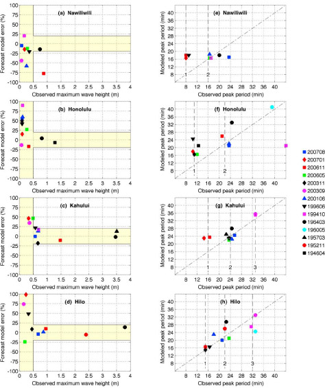
Fig. 10. (a–d) Error of the maximum wave height and (e–h) peak wave period from observations and model results by the Nawiliwili, Honolulu, Kahului, and Hilo forecast models. Forecast model error is (H − Hobs)/Hobs, where H is the modeled maximum wave height and Hobs is the observation. Colors represent subduction zones of the earthquakes. Red, central Kuril and Kamchatka; magenta, Hokkaido and west Kuril; black, Aleutian and Alaska; green, Tonga; blue, Peru; cyan, Chile.
Tsunami waves are known to produce time series with complex frequency structure that varies in space and time. To explore the tsunami frequency responses at different forecast sites, a complex Morlet wavelet transform was applied to both observations and model results. A description of the time series of wavelet-derived amplitude spectra is given by Tang et al. [2008a]. As an example, Figure 11 shows the real parts of the wavelet-derived amplitude spectra for the observation and the forecast at Hilo for the November 2006 Kuril Islands tsunami. The modulated spectrogram shows the first incident wave has a peak period near 20 min (Figure 11b). Quickly the tsunami excited two major oscillations with near 15 and 32 min periods in Hilo Harbor. Those changes of frequency structure were correctly captured by the forecast time series computed by the Hilo forecast model (Figure 11c).
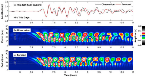
Fig. 11. (a) Time series of observed and forecast wave amplitudes at Hilo tide gauge computed by the Hilo forecast model in real time during the November 2006 Kuril Islands tsunami. Real parts of the wavelet-derived amplitude spectra of the (b) observed and (c) modeled tsunami waves are plotted.
The same approach was applied to the tsunami time series in Figure 9. Figures 10e–10h compare the observed and modeled peak wave periods at Nawiliwili, Honolulu, Kahului and Hilo. At Hilo, the observed peak wave periods fall into one of the three groups near 15, 22 or 32 min period (±2 min) (Figure 10h). The Hilo forecast model produced the peak wave periods reasonably well, especially in the highest frequency group (15 min period).
Similar to Hilo, at Kahului, the observed peak wave periods also fall into one of the three groups near 16, 24 or 32 min period (±2 min) (Figure 10g). The Kahului forecast model correctly reproduced the peak wave periods within groups 2 and 3. Although the modeled group 1 period does show up in the amplitude spectra for the 2006 and 2007 Kuril Islands tsunamis [Tang et al., 2008b], unlike the observations, it is not the dominant signal. The deep ocean tsunami observations at DART buoys for these two events show high frequency components appear in the later wave chains, which were not so well resolved in the propagation models. This may cause the peak period computed by the Kahului forecast model shifted from group 1 to group 2.
Honolulu Harbor has relatively complex geometry and tsunami waves can reach Honolulu tide station from both east and west harbor entrances. With relatively low signal-to-noise ratio data, Figure 10f shows wide range of the peak wave periods at the station. There are two distinct resonant oscillations near 11 and 22 min.
The relatively enclosed geometry of Nawiliwili Harbor produces a distinct, high natural frequency, making it different from the other three Hawaiian sites. The Nawiliwili forecast model produces the 16 min period well, and the 8 min period less well, leading to some uncertainty in forecasting such an event. The largest model-observation discrepancy in the maximum wave height was the 2006 Kuril Islands tsunami, with a 20 cm modeled maximum wave height for an 87 cm observation. The 1/3 arc sec (10 m) Nawiliwili reference inundation model produces a better fit with a 36 cm maximum height, yet still underestimates the later waves (Figure 9 time series 3a). Munger and Cheung [2008] also show large discrepancy between their maximum modeled and observed wave height at Nawiliwili for this event. Further investigation of this forecast site revealed the position of the tide station is right next to the cruise ship terminal where a ship, when docked, may affect the sensor. Coincidently, the Norwegian Star cruise ship started her docking procedures after the arrival of the first two small tsunami waves (delaying the scheduled arrival due to tsunami warning), potentially affecting the station recording. Although the exact effect of the ship interference with the tsunami signal has not been fully studied, the fact of additional data complexity at Nawiliwili is obvious.
Figures 10e–10h show that the peak wave period can be one of the local resonant periods. An interesting question is, for a particular tsunami, which local frequency may be excited as the peak frequency? Certain sites may have clearer clues than others. For example, at Kahului, Figure 10g indicates peak periods are related to the geographic locations of the earthquakes. Tsunamis originating from nearby subduction zone earthquakes excite similar peak periods at Kahului. Both the 2006 and 2007 Central Kuril Islands tsunamis have a peak period near 16 min (group 1), while the 1994 West Kuril Islands tsunami and the nearby 2003 Hokkaido tsunami present the same peak period near 32 min (group 3). The other seven tsunamis have similar peak wave periods near 24 min (group 2). Those are additional important information that can be useful for forecast and warning purposes.
To explore the hazardous wave conditions over the entire forecast site, maximum water elevation above MHW and maximum velocity computed by the forecast models were compared with those from the reference inundation models. Figures 2h and 3c show an example of Kahului for the 2003 Rat Island tsunami. Both the reference inundation model and the forecast model produced similar patterns and values. Comparisons for other tsunamis at Kahului are given by Tang et al. [2008b].
Model sensitivity studies and test applications in the previous sections provide lessons and guidance for developing site-specific tsunami models for use in operational forecasting. They have demonstrated that for a fixed tsunami source and a well-validated numerical tsunami inundation model:
Based on the above results, procedures and testing for development of tsunami forecast models are suggested as follows:
Derive DEMs from the best available bathymetric and topographic data sources at the time of development. Convert different data to the same vertical and horizontal datum. Update DEMs when better survey data becomes available.
Within acceptable computational time limits, apply the highest resolutions and largest computational domains for the forecast models. Develop a reference inundation model with highest possible resolutions and with extended computational domains for each forecast model to provide numerical references. Include bathymetric and topographic features within or close to the forecast site in the computational domains, such as nearby islands or long narrow dunes along coastlines, to provide correct coastal boundary conditions. Extend the regional grid to deep water to receive the correct dynamic boundary conditions from the coarse propagation scenarios.
Validate both the forecast model and reference inundation model with all available historical tsunami data for the model site, including tide gauge records and inundation/runup measurements. Test sensitivity of inundation to changes of friction coefficients.
Test forecast models and reference inundation models with different scenarios of simulated tsunamis based on major subduction zone earthquakes from all possible directions relative to the study sites. Verify the forecast model results with those of the reference inundation model to ensure numerical consistency. Test forecast models for stability for up to 24 hour model run for both historical and simulated scenarios of great subduction zone tsunamis.
A tsunami hazard assessment for a model site can provide forecast guidance by determining in advance which subduction zone regions and tsunami magnitudes pose the greatest thread to the location. The validated forecast models, in combination with the forecast TSF database, provide powerful tools to address this long-term forecast.
Here, we apply our forecast modeling tools, including the previously described forecast models, to produce long-term forecast assessment for Hawaiian locations. 6197 tsunami scenarios in four different magnitudes, TMw 7.5, 8.2, 8.7 and 9.3, have been explored for this study. Modeled tsunami sources are detailed in Table 4 and results are summarized in Figure 12. Figure 12 provides an overview of maximum amplitudes at offshore points from the TSFs (propagation results 1a–1d) and results of forecast model computations (forecast model results 2a–5d) for four Hawaiian locations, Nawiliwili, Honolulu, Kahului and Hilo. The forecast model results show the most dangerous tsunami source areas for a particular site and provide an overview of potential maximum amplitudes and arrival times.
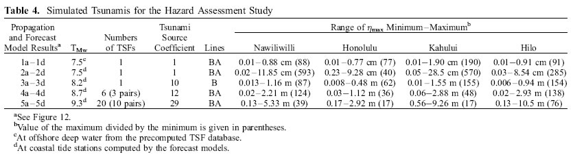
Table 4. Simulated tsunamis for the hazard assessment study.

Fig. 12. Bars in propagation results 1a–1d indicate ηmax at four offshore locations at 4400–5000 m water depth for TMw 7.5 tsunamis, which are from the TSF database. Locations of the four offshore points are shown in Figure 2a. Here ηmax at the coastal tide stations computed by the forecast models are plotted as bars at corresponding source locations in forecast model results 2a–5d for the TMw 7.5 (2a–2d), 8.2 (3a–3d), 8.7 (4a–4d), and 9.3 (5a–5d) magnitudes. Colors in forecast model results 2a–2d represent time of first tsunami arrival, t1, which is the time of water level reaching 20% height of the first significant peak or trough. Colors in forecast model results 3a–3d, 4a–4d, and 5a–5d represent the difference in time between the arrival of the maximum elevation, tmax, and the first arrival, t1.
Bars in Figure 12 propagation results 1a–1d indicate the maximum amplitude, ηmax at four offshore locations at 4400–5000 m water depth for the TMw 7.5 sources, which are from the TSF database. Locations of the four offshore points are shown in Figure 2a. The ηmax computed by the high-resolution forecast models at the coastal tide stations are plotted as bars at corresponding source locations in Figure 12 for the TMw 7.5 (forecast model results 2a–2d), 8.2 (forecast model results 3a–3d), 8.7 (forecast model results 4a–4d) and 9.3 (forecast model results 5a–5d) magnitudes. Colors represent time of first tsunami arrival, t1, which is the time of water level reaching 20% height of the first significant peak or trough. In Figure 12 forecast model results 3a–3d, 4a–4d, and 5a–5d colors represent the difference in time between the arrival of the maximum amplitude, tmax, and the first arrival, t1.
These results show an impressive local variability of tsunami amplitudes even for far-field tsunamis. The same source magnitude produces tsunami amplitudes that may be 5 times larger in Kahului than those in Honolulu. The location of the most "effective" source for a given location also differs from site to site. Even offshore tsunami amplitudes (Figure 12 propagation results 1a–1d) are not good indicators of the impact at a particular site—the intensities at tide stations (frames in lines 2 through 5) show quite different amplitude distribution. All these results illustrate the complexity of forecasting tsunami amplitudes at coastal locations. It is essential to use high resolution models in order to provide accuracy that is useful for coastal tsunami forecast.
To further investigate the transformations of tsunami amplitudes from offshore to the tide gauges, we have looked at the ratios of these amplitudes for each location. The ratio of the offshore and nearshore ηmax for all computed scenarios are plotted for the four sites and the linear regression analyses were performed in Figure 13. To better illustrate the data trends, both the logarithmic and Cartesian coordinates were plotted with the same data sets. The logarithmic scales give a full picture of the wide range of values, while the Cartesian coordinates better illustrate the actual spread and trends of the data. In Figures 13e–13h, the red dots, which represent the TMw 7.5 tsunamis, are hardly seen due to the overlapping dots representing other magnitude scenarios. The solid black lines are the best fit to the data. The dashed black lines are the prediction bounds based on 95% confidence level. The results show: (1) The relationship between tide gauge maximum amplitude and offshore maximum amplitude appears to be complex and nonlinear in nature. (2) Larger amplitudes offshore do not necessarily produce larger amplitudes at tide gauges, and larger tsunami magnitudes may not produce larger waves either offshore, or at tide gauges. (3) The trends of offshore/tide gauge amplitudes are site specific. Different sites show different regression analysis curves. (4) The simple relationships obtained through regression analysis (Figures 13a–13d) are insufficient to provide warning guidance during an event. The 95% confidence interval is too wide to provide any certainty for the forecast accuracy.

Fig. 13. Maximum computed water elevation at offshore deep water and coastal tide stations in (a–d) logarithmic and (e–h) Cartesian coordinates. Colors represent tsunami moment magnitudes. Solid lines, the fits by regression analysis in logarithmic scale; dashed lines, the prediction bounds based on 95% confident level; R, square of the correlation; RMSE, root mean squared error; p0 and p1, parameters.
These results indicate that high-resolution tsunami models are essential for providing useful accuracy for coastal amplitude forecast. If the high-resolution tsunami nearshore dynamics is not included in the forecast procedures, the accuracy and the uncertainty of the amplitude forecast appear to be too high for practical guidance.
This study describes the method and initial testing of a new forecast system built on years of effort by the whole tsunami research community. The goal of tsunami research has always been toward practical applications that will reduce the impact of this natural disaster and save lives. Real-time forecasting is an important but not the only component of this effort, which includes tsunami warning, education and community planning. This work demonstrates that a forecast, if based on direct tsunami observations and carefully designed numerical models, can finally provide accurate and timely community- and source-specific tsunami amplitude estimates for real-time tsunami assessment. This has been the goal of the tsunami research community since the first tsunami warning system was established in Japan in 1933.
The described method is only the first step in providing accurate, timely, robust and global real-time tsunami forecast. All these forecast goals (accuracy, speed, reliability, global coverage), remain formidable challenges. Our forecast research and development efforts highlighted the following outstanding gaps in the tsunami research that should be resolved in order to meet our forecasting goals.
As in several other publications [Titov, 2009; Tang et al. 2006, 2008a, 2008b; Wei et al., 2008; Titov et al., 2005], the tsunami source events discussed in this paper are far from the forecast locations. The Hawaii forecast models were chosen for demonstration because of their abundant tsunami records with relatively high signal-to-noise ratios, which is essential to assess forecast accuracy. Coastal wave amplitudes at Alaska and the U.S. West Coast for recent tsunamis (since the mid-1980s when corresponding deep ocean observations became available) are generally small and overwhelmed by noise from the continental shelf and local resonance; forecast results outside Hawaii have been published elsewhere [Wei et al., 2008; Tang et al., 2008a]. Several studies indicate, however, that the described method will be effective for local tsunami forecasting as well. The local American Samoa modeling results for the 29 September 2009 Samoa tsunami conducted at NCTR (http://nctr.pmel.noaa.gov/samoa20090929-local.html) and several recent papers [Bernard and Titov, 2007; Borrero et al., 2009] show that forecast accuracy for local events may be sufficient for critical decisions during event response. Forecast accuracy is, of course, only one component of the local tsunami problem, along with warning timing, response measures, planning, education and other factors. A thorough discussion of local forecast issues is outside of the scope of this study but will be included in several forthcoming papers at NCTR. More research is needed to evaluate this technique for local forecasting. Nevertheless, the initial results demonstrate that the method is applicable to the local tsunami problem, where not only initial tsunami arrival forecast is important, but the forecast of hours of tsunami impact is essential for critical emergency decisions during the event.
While establishing the NOAA DART network has been a huge leap in tsunami observations, and is key to tsunami forecast accuracy, questions of the optimum network size and placement of individual DARTs for best forecast accuracy require substantial additional research. DART data assimilation into forecast modeling (inversion methods) has only recently started to be researched [Percival et al., 2009] and requires substantial development. New tsunami observation methods may complement gaps in DART coverage and improve the forecast accuracy.
Assessing accuracy of the high-resolution forecast models is not easy due to limited number of observations for a particular site. New methods of assessing forecast model accuracy are needed, since there will be many forecast locations with no historical tsunami data. Model assessment of the tsunami current velocities has uncertain accuracy, due to lack of observation data. Additional research on modeling tsunami flow velocities is needed. New improved models may be required to forecast nonseismically induced tsunamis. While obviously incomplete, this list provides the immediate research needs for further forecast development.
The new forecast system not only summarizes years of research but also provides unparalleled opportunities to further tsunami science and understanding of the tsunami phenomenon. The forecast tools provide access to models, data, and a platform for testing new methods of tsunami research for future forecast application. The paper describes several research studies completed using the forecast tools with the discussion of new scientific results, in addition to the description of the development and tests of operational forecast models.
In the present study, sensitivity tests of nearshore tsunami wave characteristics were conducted for ranges of model grid setups, resolutions and parameters. Four forecast models (standby inundation models) were described for the coastal communities of Hilo, Kahului, Honolulu and Nawiliwili in Hawaii. The computational grids for the forecast models were derived from the best available bathymetric and topographic data sources. The models were tested with fourteen historical tsunamis and 6197 scenarios of simulated TMw 7.5, 8.2, 8.7 and 9.3 tsunamis based on subduction zone earthquakes in the Pacific. The outputs of the forecast models are compared to both historical water level data and numerical results from reference inundation models of higher resolution to ensure numerical consistency.
The accuracy of the maximum wave height computed by the four forecast models of 2 arc sec (60 m) resolution is greater than 80% when the observed maximum wave height is greater than 0.5 m, and the error is less than 0.3 m while the observation is less than 0.5 m. The error of the modeled first arrival is within 3% of the travel time. Wavelet analysis of the tsunami time series indicates that the peak wave period often coincides with the one of the resonant periods of the harbor where the tide gauge is located. This peak frequency may partially depend on the geographic location of the tsunami source. The optimized forecast models can accurately provide a site-specific forecast of first wave arrival time, wave amplitudes, and inundation limit within minutes of receiving tsunami source information constrained by deep ocean DART measurements. It is also capable of reproducing later tsunami waves reflected or scattered by far-field bathymetry that may arrive hours after the first arrival.
The tsunami hazard assessment study shows tsunami waves nearshore can vary significantly from the same magnitude tsunamis from different subduction zones or different locations on the same subduction zone. Furthermore, the offshore maximum wave amplitude is not a good indicator for the amplitude at a tide gauge. Therefore, earthquake magnitude alone is ambiguous and insufficient to provide information for accurate coastal tsunami amplitude forecasting. By including local bathymetry and topography and utilizing deep ocean tsunami measurement data via DART-constrained propagation scenario, which reflects the event-specific tsunami magnitude, the high-resolution forecast models are able to quickly provide accurate site-specific coastal predictions.
The authors thank the reviewers for their comments and suggestions; Elena Tolkova and Jean Newman for their extensive assistances; Mick Spillane for providing information on Kahului offshore; Marie Eble, Nazila Merati, Lindsey Waller, Clyde Kakazu and Allison Allen for assistance with tide gauge and DART data; Eddie Bernard, Yong Wei, Robert Weiss, Diego Arcas, Burak Uslu and Arun Chawla for discussions; Edison Gica for assistance with the TSF database; Christopher Moore for assistance with MOST I/O; David Borg-Breen and Doug Jongeward for hardware and software support; and Ryan L. Whitney for comments and editing. This research is funded by the NOAA Center for Tsunami Research (NCTR), PMEL contribution 3332. This publication is partially funded by the Joint Institute for the Study of the Atmosphere and Ocean (JISAO) under NOAA Cooperative agreement NA17RJ1232, contribution 1757.
Allen, A. L., N. A. Donoho, S. A. Duncan, S. K. Gill, C. R. McGrath, R. S. Meyer, and M. R. Samant (2008), NOAA's National Ocean Service supports tsunami detection and warning through operation of coastal tide stations, in Solutions to Coastal Disasters 2008 Tsunamis: Proceedings of Sessions of the Conference, April 13–16, 2008: Turtle Bay, Oahu, Hawaii, edited by L. Wallendorf et al., pp. 1–12, Am. Soc. of Civ. Eng., Reston, VA.
Berkman, S. C., and J. M. Symons (1964), The tsunami of May 22, 1960 as recorded at tide stations, Coast and Geodetic Survey Preliminary Report, 69 pp., U.S. Dept. of Comm., Washington, D.C.
Bernard, E., and V. V. Titov (2007), Improving tsunami forecast skill using deep ocean observations, Mar. Technol. Soc. J., 40(3), 23–26.
Bernard, E. N., H. O. Mofjeld, V. V. Titov, C. E. Synolakis, and F. I. González (2006), Tsunami: Scientific frontiers, mitigation, forecasting, and policy implications, Philos. Trans. R. Soc. London Ser. A, 364(1845), 1989–2007, doi:10.1098/rsta.2006.1809.
Borrero, J. C., R. Weiss, E. A. Okal, R. Hidayat, D. Arcas, and V. V. Titov (2009), The tsunami of 2007 September 12, Bengkulu province, Sumatra, Indonesia: Post-tsunami field survey and numerical modeling, Geophys. J. Int., 178, 180–194, doi:10.1111/j.1365–246X.2008.04058.x.
Geist, E. L., V. V. Titov, and C. E. Synolakis (2006), Tsunami: Wave of change, Sci. Am., 294, 56–65.
Gica, E., M. C. Spillane, V. V. Titov, C. D. Chamberlin, and J. C. Newman (2008), Development of the forecast propagation database for NOAA's Short-Term Inundation Forecast for Tsunamis (SIFT), Tech. Memo. OAR PMEL–139, 89 pp., Gov. Print. Off., Seattle, WA.
González, F. I., E. N. Bernard, C. Meinig, M. Eble, H. O. Mofjeld, and S. Stalin (2005), The NTHMP tsunameter network, Nat. Hazards, 35(1), 25–39.
Green, C. K. (1946), Seismic sea wave of April 1, 1946, as recorded on tide gauges, Eos Trans. AGU, 27, 490–500.
Greenslade, D. J. M., M. A. Simanjuntak, and D. Burbidge (2007), A first-generation real-time tsunami forecasting system for the Australian Region, Res. Rep. 126, 84 pp., Bur. of Meteorol., Melbourne, Victoria, Australia.
Gusiakov, V. K. (1978), Static displacement on the surface of an elastic space, in Ill-Posed Problems of Mathematical Physics and Interpretation of Geophysical Data (in Russian), pp. 23–51, Comput. Cent. of Sov. Acad. of Sci., Novosibirsk, Russia.
Johnson, J. M., and K. Satake (1999), Asperity distribution of the 1952 Great Kamchatka earthquake and its relation to future earthquake potential in Kamchatka, Pure Appl. Geophys., 154(3–4), 541–553, doi:10.1007/s000240050243.
Johnson, J. M., Y. Tanioka, L. J. Ruff, K. Satake, H. Kanamori, and L. R. Sykes (1994), The 1957 Great Aleutian Earthquake, Pure Appl. Geophys., 142(1), 3–28, doi:10.1007/BF00875966.
Johnson, J. M., K. Satake, S. R. Holdahl, and J. Sauber (1996), The 1964 Prince William earthquake: Joint inversion of tsunami and geodetic data, J. Geophys. Res., 101(B1), 523–532, doi:10.1029/95JB02806.
Kanamori, H., and J. J. Ciper (1974), Focal process of the great Chilean earthquake, May 22, 1960, Phys. Earth Planet. Inter., 9, 128–136, doi:10.1016/0031-9201(74)90029-6.
Kuwayama, T. (2007), Quantitative tsunami forecast system, paper presented at Intergovernmental Coordination Group for the Pacific Tsunami Warning and Mitigation System Tsunami Warning Centre Coordination Meeting, Intergov. Oceanogr. Comm., Honolulu, Hawaii, 17–19 Jan.
Lautenbacher, C. (2005), Tsunami warning systems, Bridge, 35, 21–25.
Liu, P. L.-F. (2009), Tsunami modeling-Propagation, in The Sea, vol. 15, edited by E. Bernard and A. Robinson, chap. 9, pp. 295–319, Harvard Univ. Press, Cambridge, MA.
López, A. M., and E. A. Okal (2006), A seismological reassessment of the source of the 1946 Aleutian 'tsunami' earthquake, Geophys. J. Int., 165(3), 835–849, doi:10.1111/j.1365-246X.2006.02899.x.
Munger, S., and K. F. Cheung (2008), Resonance in Hawaii waters from the 2006 Kuril Islands Tsunami, Geophys. Res. Lett., 35, L07605, doi:10.1029/2007GL032843.
National Geophysical Data Center (2007), Historical Tsunami Database, http://www.ngdc.noaa.gov/hazard/tsu_db.shtml, Boulder, Colo.
National Science and Technology Council (2005), Tsunami risk reduction for the United States: A framework for action, report, 30 pp., Washington, D.C.
Nayak, S., and T. S. Kumar (2008), Indian tsunami warning system, Int. Arch. of Photogramm. Remote Sens., 37, 1501–1506.
Okada, Y. (1985), Surface deformation due to shear and tensile faults in a half-space, Bull. Seismol. Soc. Am., 75, 1135–1154.
Pararas-Carayannis, G. (1969), Catalog of Tsunamis in The Hawaii Islands, 94 pp., U.S. Dept. of Commer., Washington, D.C.
Percival, D. B., D. Arcas, D. W. Denbo, M. C. Eble, E. Gica, H. O. Mofjeld, M. C. Spillane, L. Tang, and V. V. Titov (2009), Extracting tsunami source parameters via inversion of DART® buoy data, Tech. Memo. OAR PMEL–144, 22 pp., Gov. Print. Off., Seattle, WA.
Rudloff, A., U. Muench, and J. Lauterjung (2008), Launch of the German Indonesian Tsunami Early Warning System (GITEWS), Eos Trans. AGU, 89(53), Fall Meet. Suppl., Abstract OS42B–02.
Salsman, G. G. (1959), The tsunami of March 9, 1957, as recorded at tide stations, Coast Geod. Surv. Tech. Bull. 6, 18 pp., U.S. Gov. Print. Off., Washington, D.C.
Satake, K., Y. Hasegawa, Y. Nishimae, and Y. Igarashi (2008), Recent tsunamis that affected the Japanese coasts and evaluation of JMA's tsunami warnings, Eos Trans. AGU, 89(53), Fall Meet. Suppl., Abstract OS42B–03.
Shepard, F. P., G. A. Macdonald, and D. C. Cox (1950), Tsunami of April 1, 1946, Bull. Scripps Inst. Oceanogr., 5, 391–528.
Smith, W. H. F., and D. T. Sandwell (1997), Global seafloor topography from satellite altimetry and ship depth soundings, Science, 277, 1957–1962.
Sobolev, S. V., A. Y. Babeyko, R. Wang, R. Galas, M. Rothacher, D. Stein, J. Schröter, J. Lauterjung, and C. Subarya (2006), Towards real-time tsunami amplitude prediction, Eos Trans. AGU, 87(37), 374, 378.
Spaeth, M. G., and S. C. Berkman (1967), The tsunami of March 28, 1964, as recorded at tide stations, Coast Geod. Surv. Tech. Bull. 33, 86 pp., U.S. Dept. of Comm., Rockville, MD.
Synolakis, C. E., and E. N. Bernard (2006), Tsunami science before and beyond Boxing Day, Philos. Trans. R. Soc. London Ser. A, 364, 2231–2265.
Synolakis, C., E. Okal, and E. N. Bernard (2005), The megatsunami of December 26, 2004, Bridge, 35, 26–35.
Synolakis, C. E., E. N. Bernard, V. V. Titov, U. Kânoğlu, and F. I. González (2008), Validation and verification of tsunami numerical models, Pure Appl. Geophys., 165(11–12), 2197–2228, doi:10.1007/s00024-004-0427-y.
Tang, L., C. D. Chamberlin, E. Tolkova, M. Spillane, V. V. Titov, E. N. Bernard, and H. O. Mofjeld (2006), Assessment of potential tsunami impact for Pearl Habor, Hawaii, Tech. Memo. OAR PMEL–131, 36 pp., Gov. Print. Off., Seattle, WA.
Tang, L., V. V. Titov, Y. Wei, H. O. Mofjeld, M. Spillane, D. Arcas, E. N. Bernard, C. D. Chamberlin, E. Gica, and J. Newman (2008a), Tsunami forecast analysis for the May 2006 Tonga tsunami, J. Geophys. Res., 113, C12015, doi:10.1029/2008JC004922.
Tang, L., C. D. Chamberlin, and V. V. Titov (2008b), Developing tsunami forecast inundation models for Hawaii: Procedures and testing, Tech. Memo. OAR PMEL–141, 46 pp., Gov. Print. Off., Seattle, WA.
Tang, L., V. V. Titov, and C. D. Chamberlin (2009), A tsunami forecast model for Hilo, Hawaii, PMEL Tsunami Forecast Ser., vol. 1, 44 pp., Gov. Print. Off., Seattle, WA.
Titov, V. V. (2009), Tsunami forecasting, in The Sea, vol. 15, Tsunamis, chap. 12, edited by E. N. Bernard and A. R. Robinson, pp. 371–400, Harvard Univ. Press, Cambridge, MA.
Titov, V. V., and F. I. González (1997), Implementation and testing of the Method of Splitting Tsunami (MOST) model, Tech. Memo. ERL PMEL 112, 11 pp., Gov. Print. Off., Seattle, WA.
Titov, V. V., and C. S. Synolakis (1998), Numerical modeling of tidal wave runup, J. Waterw. Port Coastal Ocean Eng., 124(4), 157–171, doi:10.1061/(ASCE)0733-950X(1998)124:4(157).
Titov, V. V., H. O. Mofjeld, F. I. González, and J. C. Newman (1999), Offshore forecasting of Alaska-Aleutian subduction zone tsunamis in Hawaii, Tech. Memo. ERL PMEL–114, 22 pp., Gov. Print. Off., Seattle, WA.
Titov, V. V., H. O. Mofjeld, F. I. González, and J. C. Newman (2001), Offshore forecasting of Alaskan tsunamis in Hawaii, in Tsunami Research at the End of a Critical Decade, edited by G. T. Hebenstreit, pp. 75–90, Kluwer Acad., Dordrecht, Netherlands.
Titov, V. V., F. I. González, E. N. Bernard, M. C. Eble, H. O. Mofjeld, J. C. Newman, and A. J. Venturato (2005), Real-time tsunami forecasting: Challenges and solutions, Nat. Hazards, 35(1), 41–58.
Wei, Y., E. Bernard, L. Tang, R. Weiss, V. Titov, C. Moore, M. Spillane, M. Hopkins, and U. Kânoğlu (2008), Real-time experimental forecast of the Peruvian tsunami of August 2007 for U.S. coastlines, Geophys. Res. Lett., 35, L04609, doi:10.1029/2007GL032250.
Whitmore, P. M. (2003), Tsunami amplitude prediction during events: A test based on previous tsunamis, Sci. Tsunami Hazards, 21, 135–143.
Zerbe, W. B. (1953), The tsunami of November 4, 1953 as recorded at tide stations, Coast Geod. Surv. Tech. Bull. 300, 62 pp., U.S. Dept. of Comm., Washington, D.C.
Return to Abstract