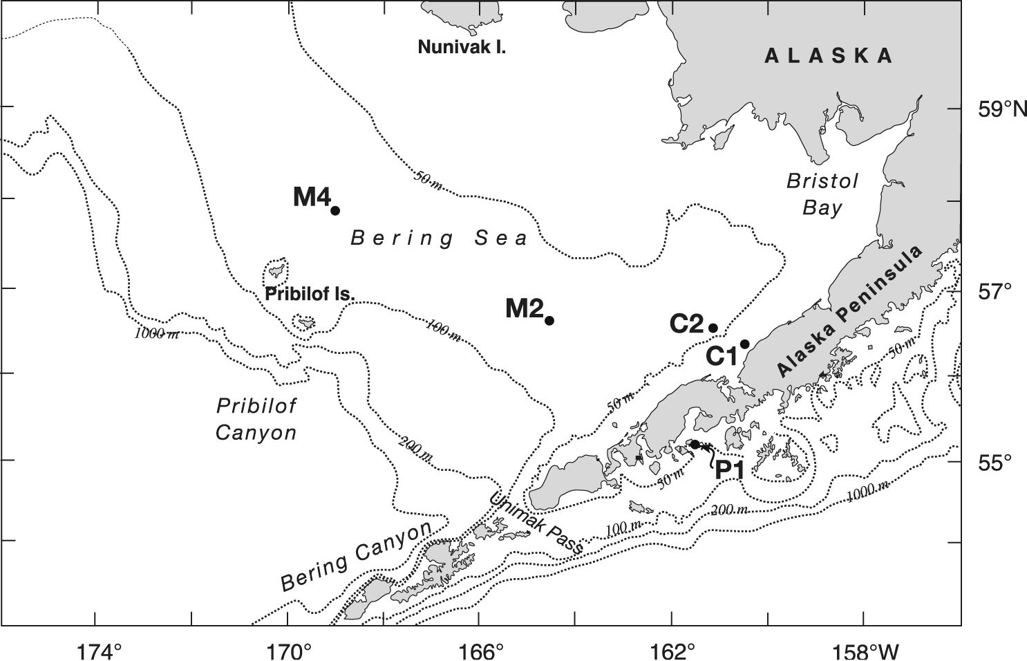
Fig. 1. Location map of the southeastern Bering Sea shelf showing the 50, 100, 200, and 1000 m isobaths. The locations of the five mooring sites discussed in the manuscript are shown.
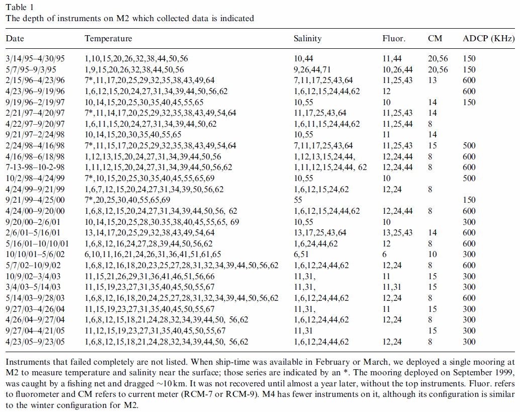
Table 1.
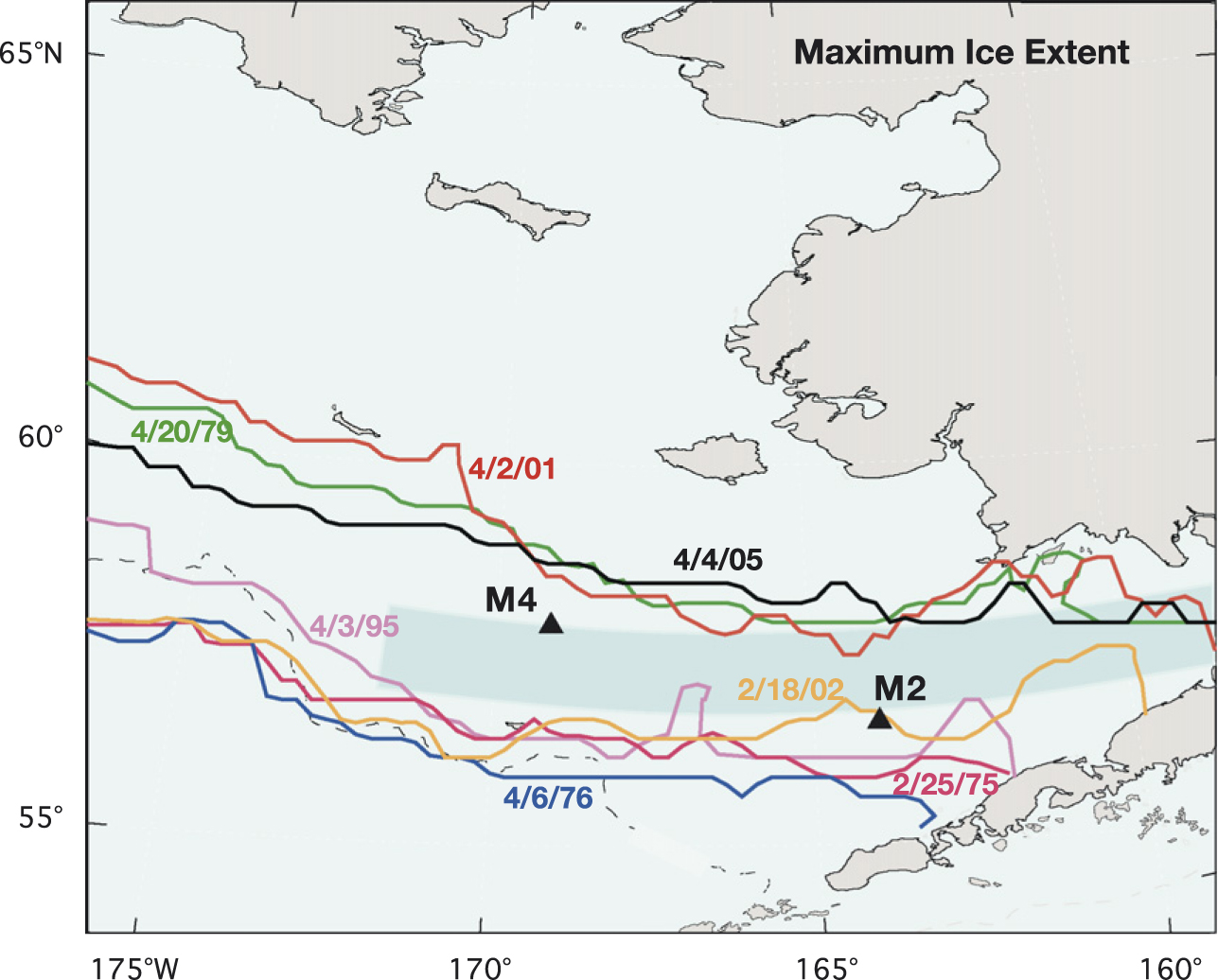
Fig. 2. Maximum ice extent (45% concentration) during selected years as discussed in the paper. The locations of M2 and M4 are indicated as triangles. The shaded area is the box where ice concentrations shown in Fig. 3 were calculated.
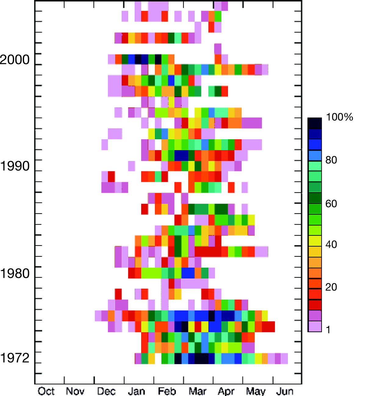
Fig. 3. Percent ice cover from 57°N to 58°N (the shaded area in Fig. 2). Each square represents 1 week.
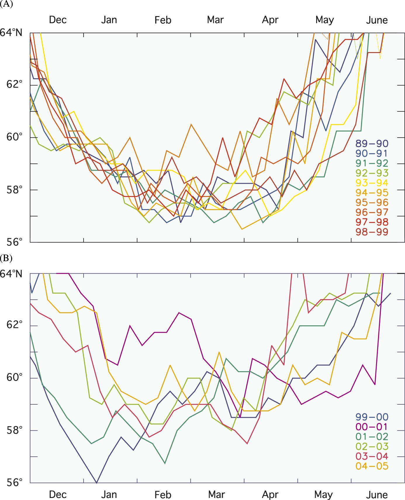
Fig. 4. The southernmost latitude of sea ice along 169°W during each week from December to June. The upper panel represents the ‘‘cool period’’ years from 1989 to 1999 and the bottom panel the warmer period that has dominated the system during the last 5–6 years.
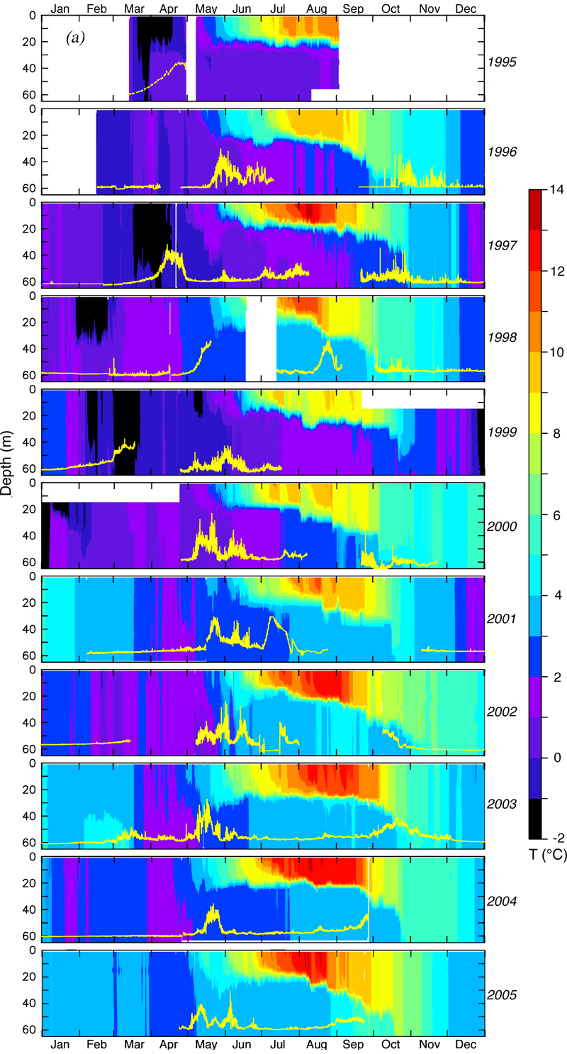
Fig. 5. (A) Contours of temperature measured at M2. The coldest temperatures (black) occurred when ice was over the mooring. The temperature contours have been extended to the surface from 10m during winter (October–March) period as discussed in the text. The yellow line is fluorescence measured at ~11 m. Note that early blooms are associated with the presence of ice. (B) Contours of temperature measured at M4. The coldest temperatures (black) occurred when ice was over the mooring. The temperature contours have been extended to the surface from ~10 m as discussed in the text. The yellow line is fluorescence measured at ~11 m. Note that early blooms are associated with the presence of ice.
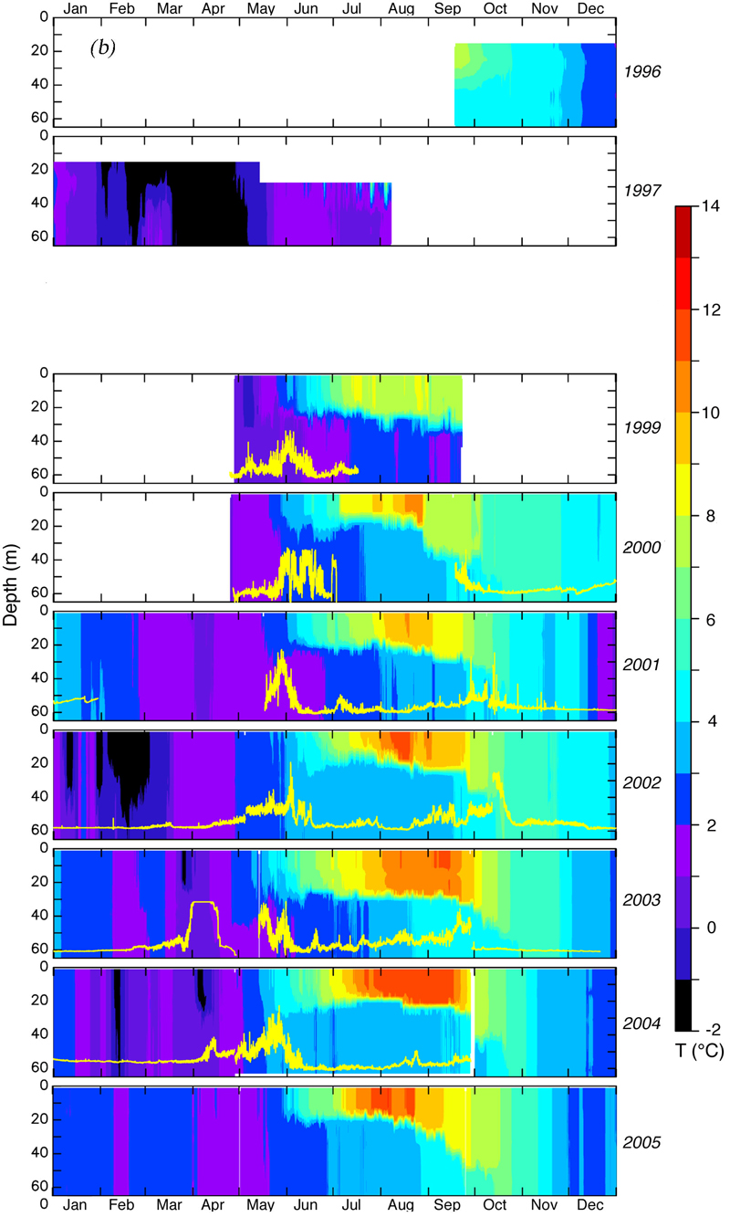
Fig. 5. (Continued)
Fig. 6. (A) Depth-averaged temperature at M2 and M4. (B) The difference between depth-averaged temperatures at M2 and M4. The depth-averaged temperature anomaly (the seasonal signal has been removed) at (C) M2 and (D) M4. All time series have been low-passed filtered.
![]()
Fig. 7. Near bottom temperatures at the two moorings in Bristol Bay. C1 is in 20 m of water and C2 in 60 m. The time series have been low-pass filtered.
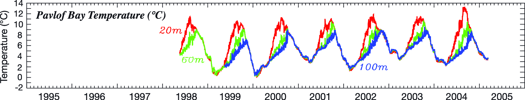
Fig. 8. Temperature at three depths (20, 60, and 100 m) at the entrance to Pavlof Bay in the Gulf of Alaska (P1 in Fig. 1). The time series have been low-pass filtered.
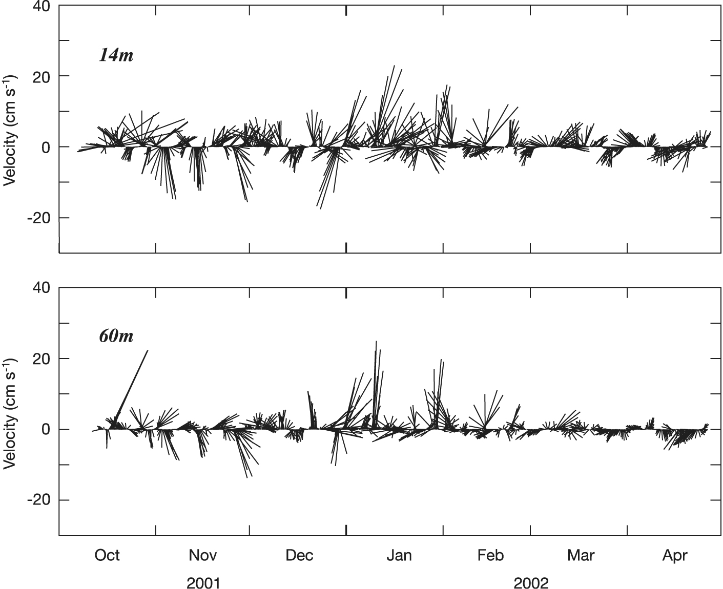
Fig. 9. Low-pass filtered current velocity measured at 14 and 60 m depth at M2. Up is northward flow.
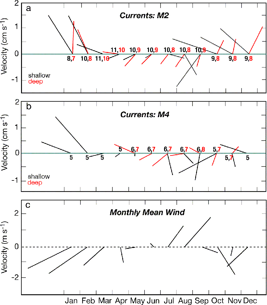
Fig. 10. The mean monthly current velocity (A) at M2 and (B) at M4. The shallow currents were measured at depths of 8–12 m and the deep currents were measured at 55–65 m. The numbers along the axis indicate the number of years that there were data during that month. (C) The NCEP reanalysis wind velocity has been interpolated to the position of M2. Up is northward flow.

Fig. 11. Mean 700 hPa geopotential height anomaly (m) for (top panel) December 1974–March 1975 and (bottom panel) for December 2001–March 2002. Anomalies are relative to a baseline period of 1968–1996.
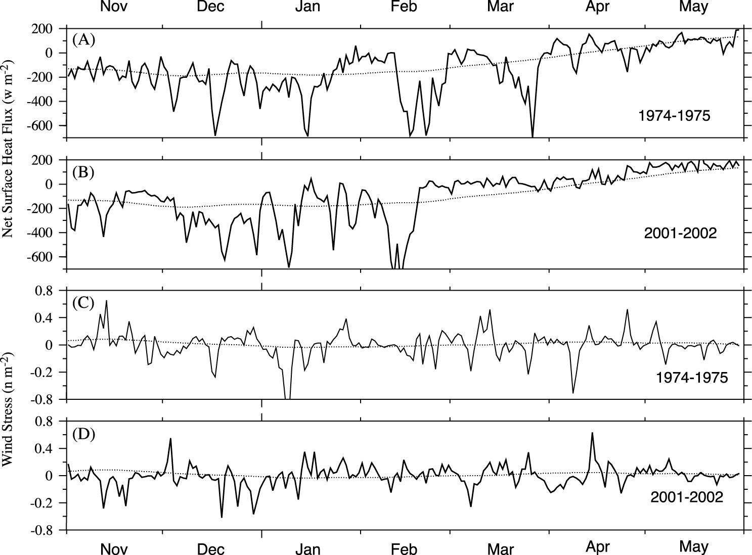
Fig. 12. Daily values of the net surface heat flux (W m2) at (A) Site 2 (57°N, 164°W) and (B) at Unimak Pass (54°N, 165°W). Panels (C) and (D) show the along-peninsula wind stress (N m2) for the same locations for 1 November 1974–31 May 1975. Negative is toward the west-southwest. The dotted lines represent climatological means.
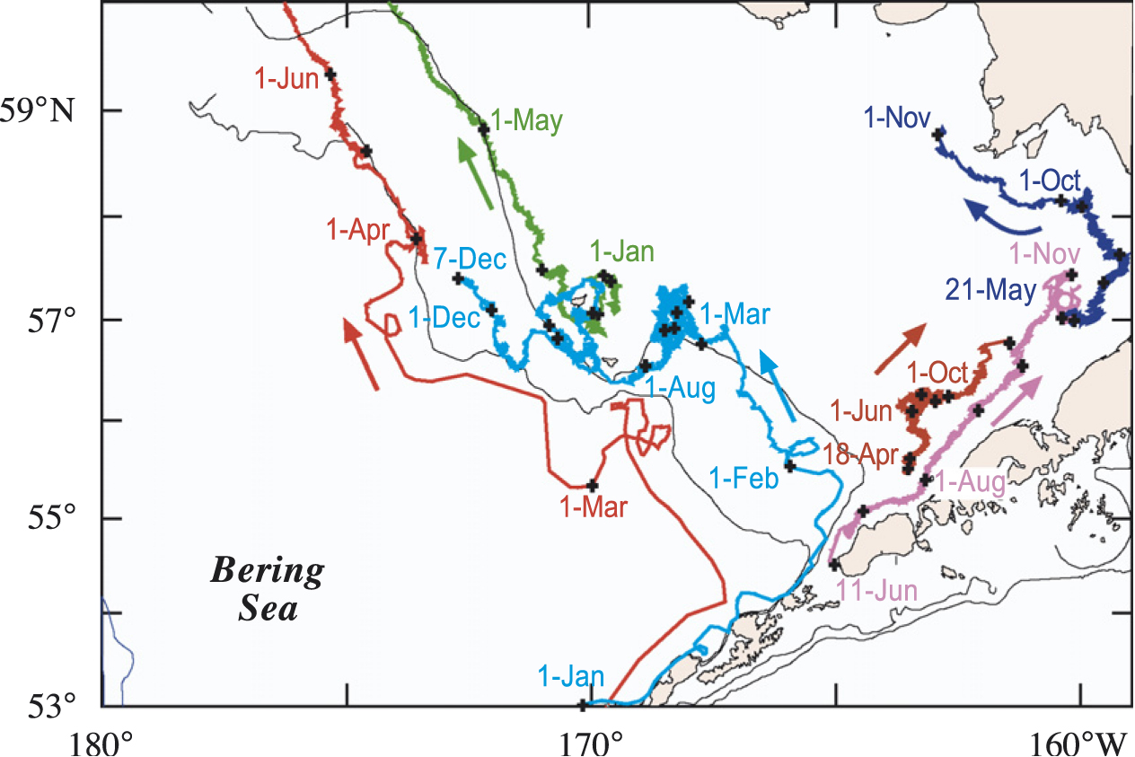
Fig. 13. Satellite-tracked drifter trajectories. The black "+" indicate the position of the drifter at the first of each month. The drifters each had "holey sock" drogues centered at ~40 m depth.
Return to References
Return to Abstract