Features of the physical environment of the eastern Bering Sea (Fig. 1) — including length of day, net short-wave radiation flux (Overland et al., 2001), wind fields, ice cover, on/off shelf transport, water column structure and temperature — change with rhythms spanning a broad frequency spectrum. As a high-latitude sea, most of the physical features exhibit a strong seasonal signal as well as longer-period fluctuations ranging from year-to-year, to decadal, to trends forced by climate change (Schumacher and Alexander, 1999). Such changes in climate are mechanistically transmitted through the ocean to biota (e.g. Francis et al., 1998). Over the south-eastern shelf, the year-to-year variation in ice extent, which has ramifications for oceanic characteristics and biota, provides a mechanism not present in more temperate ecosystems. The extent and timing of sea ice cover can dramatically alter the time/space characteristics of primary/secondary production (Niebauer et al., 1995, 1990; Niebauer and Day, 1989; Stabeno et al., 1999), and hence food for larval fishes (Napp et al., 2000). Fish distributions (Wyllie-Echeverria and Wooster, 1998) and survival of age-1 pollock (Ohtani and Azumaya, 1995) respond to the extent of the cold pool of bottom water over the shelf, which is closely related to the maximum extent of ice cover. A massive increase in jellyfish population over the eastern shelf has been linked to climate change through the atmosphere's influence on ice cover (Brodeur et al., 1999).
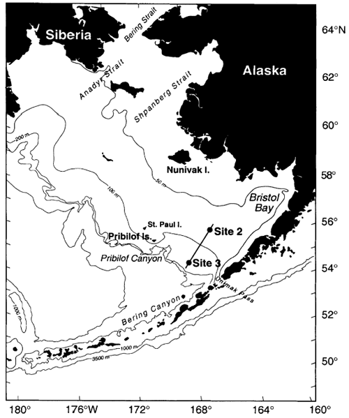
Figure 1. Geography and place names in the eastern Bering Sea. The location of the two mooring sites is indicated by bold numerals. The hydrographic transect is shown as a solid line. Depth contours are in metres.
Understanding the south-eastern Bering Sea is of particular importance because it is the most productive marine ecosystem in the United States and one of the most productive in the world. Besides the lucrative king crab, halibut, and salmon fisheries, most of the world's catch of walleye pollock comes from the Bering Sea. Historically, marked changes in the ecosystem have occurred that resulted in changes in nodal species (e.g. National Research Council, 1996). Any change to this rich ecosystem that causes a reduction in productivity, change in species composition, or change in the portion of the food web that is usable by mankind, will have a severe societal impact. Fluctuations in the physical environment can adversely affect the ecosystem both through changes in the nutrient-phytoplankton-zooplankton sequence (bottom-up control), and by altering habitat, which results in changes in abundance and composition of higher-trophic-level animals (top-down control). Interannual variability in the atmosphere and in the ocean's response have significant implications for the biota, as shown for the North Pacific by Mantua et al. (1997). For the eastern Bering Sea, top-down control may be responsible for year-to-year fluctuation of zooplankton and phytoplankton biomasses, while bottom-up control has been suggested as the mechanism for longer period (decadal) variations (Sugimoto and Tadokoro, 1997). To advance our understanding of how the Bering Sea ecosystem functions requires monitoring the environment, identifying the important fluctuations, and elucidating the mechanisms by which changes in physical phenomenon are transferred to biota.
The Bering Sea experienced a variety of anomalous conditions during 1997 and 1998 (Stabeno, 1998; Vance et al., 1998; Napp and Hunt, 2001), including: major coccolithophorid blooms (1997 and 1998), a large die-off of shearwaters (1997; Baduini et al., 2001), salmon returns far below predicted numbers (1997 and 1998), the presence of whales in the waters of the middle shelf (1997 and 1998), unusually warm sea surface temperatures (1997 and 1998), and a decrease in the onshore transport of slope water (1997). The causal mechanisms for these events are not completely understood, but major shifts in the ecosystem have occurred in the past, and we may now be witnessing such an event.
To place the changes observed in 1997 and 1998 in context with past variability of this ecosystem, a careful examination of historical data is necessary to establish baseline characteristics of the physical environment. In the first section of this paper we discuss the factors controlling the atmospheric forcing and how 1997 and 1998 fit into the historical record. We then examine the spatial patterns and temporal variability of sea ice over the Bering Sea shelf. Next we address the variability in the currents, temperature and salinity at two sites on the Bering Sea shelf where long-term moorings have been maintained (1995-1998). Hydrographic data collected since 1966 along a transect and at the mooring sites are analysed and interpreted with focus on the conditions in 1997 and 1998. We conclude by discussing the implications that the observed changes may have on this ecosystem in the future.
The direct effects of atmospheric forcing are crucial to the dynamics of the south-eastern Bering Sea. Because the mean flow over the shelf tends to be sluggish, and any direct oceanographic connection between the shelf and the North Pacific is obstructed by the Alaska Peninsula, the linkages between the south-eastern Bering Sea and the climate system are largely mediated by the atmosphere. Given the basin-wide scale of the atmospheric anomalies that dominate the seasonal and longer-term variability, the conditions that occurred in the south-east Bering Sea in 1997-1998 are related to the state of the entire North Pacific climate system. Previous work on this climate system concentrated on the wintertime atmospheric forcing and oceanic response (Miller et al., 1994; Trenberth and Hurrel, 1994), but interest in spring and summer conditions is increasing (e.g. Overland et al., 2001). Here we take a somewhat broader and less detailed view and consider both the winter and summer conditions during 1997 and 1998, and compare them to their climatological norms.
The atmospheric forcing of the south-east Bering Sea during winter is substantial, and through the long-lasting effects of sea ice, its influence can persist through the summer. The atmospheric circulation over the North Pacific and Bering Sea features large interannual fluctuations. It is important to recognize that this circulation is inherently variable on time scales longer than a few days, and much of this variability defies simple explanation. Nevertheless, frameworks do exist for accounting for some aspects of the variability. Most notable are the correlations between the North Pacific circulation and the El Niño-Southern Oscillation (ENSO) (Horel and Wallace, 1981) which varies on 2-7 year time scales, and the Pacific Decadal Oscillation (PDO) of North Pacific sea surface temperature (Mantua et al., 1997), which varies on decadal time scales. Figure 2 shows time series for ENSO (in terms of the NINO3 index) and the PDO, and their relationship to a more direct parameter for the Bering Sea, namely, the strength of the seasonal mean Aleutian Low. The strength (and position) of the Aleutian Low is important to the Bering Sea through its impact on the winds and surface heat fluxes, which in turn affect the formation and advection of sea ice. In general, deep, strong Aleutian Lows are associated with warmer-than-normal winters in the south-eastern Bering Sea, because the individual storm systems preferentially pump warm air poleward. On the other hand, weaker Aleutian Lows tend to be associated with an abundance of migrating anticyclones, which usually transport cold air equatorward. The effects of these transients can be modulated by the mean meridional wind anomalies that can also accompany changes in the position and strength of the Aleutian Low. Both the NINO3 and PDO indices underwent a marked change in the mid-late 1970s; this is the 'regime shift' noted by Trenberth (1990) and others. These time series (Fig. 2) reveal that the Aleutian Low is generally stronger when the NINO3 and especially the PDO indices are positive, and vice versa. The Aleutian Low during 1996, 1997 and 1998 was slightly stronger than normal, while during 1995 it was weaker (Fig. 2). This variability contributed to substantial differences in the timing and duration in the sea ice over the Bering Sea shelf, as will be shown in the following section.
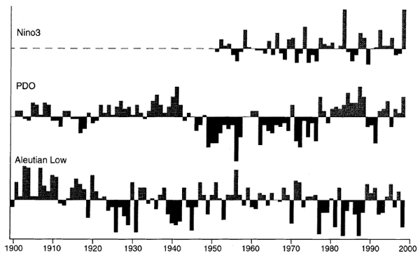
Figure 2. Time series for ENSO (the NINO3 index), the PDO8 (after Mantua et al., 1997), and the Aleutian Low.
Mooring measurements have been collected on the shelf from 1995 to 1998 (see following sections) and can be used to examine the response of the south-east Bering Sea to a variety of wintertime conditions. For summertime, we have examined atmospheric forcing during 1997 and 1998 in the context of the historical record. This analysis complements the results of Overland et al. (2001), which focused on the anomalous heating during the summer of 1997 and its links to the 1997-1998 El Niño. As mentioned above, the bulk of previous research on the atmospheric circulation over the North Pacific has concentrated on the winter season. Its variability has been characterized in terms of preferred modes, such as the Pacific-North American pattern (PNA). The atmospheric variability is weaker in the summer, but it can also be characterized in terms of a small number of modes, which can differ from their winter counterparts. (For a general summary of these modes and their calculation, see Barnston and Livezey, 1987.)
The primary mode for the south-east Bering Sea from the spring to early summer is generally the North Pacific (NP) pattern. This mode consists of a dipole in tropospheric pressure anomalies between (roughly) northern Alaska and the west central Pacific along 40°N. Two other modes that flank the NP, the West Pacific (WP) and East Pacific (EP) patterns, are also prominent during the early and middle stages of the warm season, respectively. As shown by Overland et al. (2001), the NP and EP indices have been systematically positive and negative, respectively, since about 1990. Both modes have contributed to anomalously high pressures that have occurred over Alaska during the warm season for the last decade. During the spring and summer the WP was systematically negative (i.e. contributing towards higher pressure over the central Bering Sea) from the early 1980s to about 1990.
The large-scale pressure anomalies that comprise these modes are important to the south-east Bering Sea through their modulation of the processes that determine air-sea interaction. During the warm season, the two most important aspects of atmospheric forcing are the magnitude of solar radiation and wind speed at the sea surface. The incident solar radiation, together with mixed layer depth, controls the heating of the upper ocean during the summer; the wind speed regulates the depth of the mixed layer and the turbulent exchange at the base of the upper mixed layer, and hence the distribution of this heat in the water column.
Solar heating anomalies were strongly positive in 1997, especially from late May to mid-July (Overland et al., 2001), but were near zero in 1998 (not shown). These anomalies have been systematically positive since the early 1980s, and were systematically negative from the late 1950s to the early 1970s. Winds during the warm season, as indicated by observations at St. Paul Island in the Pribilof Islands (Fig. 3), were weak in 1997, with the exception of one prominent event in May. In 1998, winds were strong into June and after mid-August. By way of comparison, the winds in 1995 (1996) tended to be weaker (stronger) than typical. In general, the warm-season winds have tended to be weaker than their climatological norms since the early 1980s.
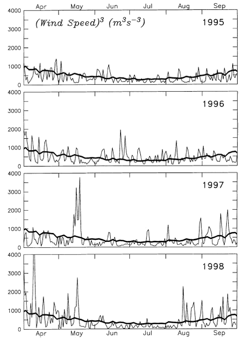
Figure 3. Times series of wind speed cubed (an indicator of the strength of wind mixing) measured at St Paul Island, 1995-1998. The bold line in each panel is the smoothed (3 day running average) daily mean value established from the 48 year long data set.
One of the defining characteristics of the eastern Bering Sea shelf is an annual advance and retreat of sea ice. Ice formation begins as early as November and can remain over the south-eastern shelf into June. The juxtaposition of the Aleutian Low and Siberian High typically produces winter winds from the north-east, freezing the sea water and pushing the resulting ice south-westward. Owing to fluctuations in these winds and in air temperature, large (hundreds of kilometres) interannual variability in the annual maximum extent of sea ice exists. The advection and eventual melting of ice play a critical role in the fluxes of heat and salt. The leading edge of the ice is continuously melting, introducing cold (about -1.7°C), relatively fresh water into the water column. Extensive mixing of the water column can occur beneath the moving ice, which overcomes the positive buoyancy (fresh water) produced by melting. Over the middle shelf, this mixing can extend to >80 m during periods of strong winds. The introduction of cold water throughout the water column results in the creation of a cold lower layer. As the surface warms from spring-summer heating, this isolates the cold bottom water, resulting in a feature known as the cold pool. This layer is 40-50 m thick with temperatures below 2°C, which persists through the summer, often warming only slightly.
These coupled atmosphere-ocean mechanisms have a significant influence on biota. An ice-edge phytoplankton bloom occurs in the marginal ice zone during the spring (Niebauer et al., 1990; Niebauer et al., 1995) and produces a large fraction (up to 65%) of the annual primary production over the shelf. The sequence of nutrients to phytoplankton to zooplankton appears to be critical for providing food to first feeding pollock larvae (Napp et al., 2000).
The timing of ice cover varies greatly among years. We obtained the position of the ice edge from the compact disk produced by the National Ice Center, the Fleet Numerical Meteorology and Oceanography Detachment, and the National Climatic Data Center. This data set contains information on the ice concentration and thickness from weekly satellite images from 1972 through 1994. For the data since 1994, we digitized the Alaska Regional Ice Charts, which are produced by the Anchorage Forecast Office of the National Weather Service.
We focus our analysis of the temporal variability of sea ice on the middle shelf near Site 2 (Fig. 1). At this location, we have collected temperature, salinity, nutrient, fluorescence and other parameters since 1995 (discussed later in this article). The time of arrival, departure and the persistence of sea ice at this location (Fig. 4) indicates that years with the most extensive ice coincided with a strong negative PDO (Fig. 2). Sea ice has arrived at this location as early as January and remained as late as mid-May. Between 1979 and 1981, ice was largely absent from the middle shelf near Site 2. These were years when extensive water property observations were collected as part of PROBES (Coachman, 1986); these observations led to much of the present understanding of characteristics and processes over this shelf. Beginning in the early 1990s, sea ice once again became more common in this region, although not to the extent observed in the early 1970s. Neither the PDO nor ENSO accounts for all the fluctuations in sea ice over this region. In particular, the manifestation of El Niño at high latitudes is not consistent. There was no ice at Site 2 during two of the five El Niño events that occurred since 1972 (Fig. 4), and the presence of ice during other years was intermittent. These characteristics are not, however, uncommon to this time series; ice was also intermittent or absent in non-El Niño years. These results are consistent with Niebauer et al. (1999), who found only a weak negative correlation between ENSO and sea ice extent.
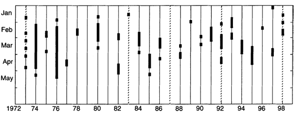
Figure 4. The timing of arrival and departure of sea ice at Site 2 is indicated by the dark bars. Dotted vertical lines indicate periods when an El Niño was occurring on the equator.
To characterize the temporal variability in the spatial pattern of sea ice (Fig. 5), we divided the time series of ice observations into three subsets based on the regime shifts (Ohtani and Azumaya, 1995; Trenberth and Hurrell, 1995). These are 1972-1976 (cold period), 1977-1988 (warm period), and 1989-1998 (cool period). A marked difference exists in persistence and spatial distribution of ice between the first (cold) period and the latter two periods. During the first period, ice covered the shelf out to and over the upper slope and remained around St. Paul Island for more than a month. During the later years, ice did not extend as far seaward, and its residence time was typically 2-4 weeks less than during the cold period. The differences between the two latter regimes are more subtle, but still evident. Along 59°N, during 1989-1998, there were 2-4 weeks more ice than during 1977-1988. Surprisingly, north of St. Lawrence Island and along the west coast of Alaska north of Nunivak Island, there were 1-2 more weeks of ice cover in the warm period than in the cooler, third period. This resulted from either later arrival or more rapid retreat of sea ice over the northern Bering Sea shelf during 1989-1998, in agreement with observations from native Alaskans, who have lived in this area for generations. It should be noted that Site 2 is in a region of highly variable ice cover duration, and while ice usually reaches this location, it is often nearing its southernmost extent.
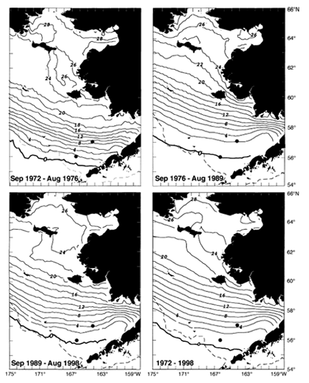
Figure 5. Contours of the number of weeks that sea ice was present over the eastern Bering Sea shelf. The average ice coverage during (a) cold period, (b) warm period, (c) cool period, and (d) 1972-1998. Solid circles denote Sites 2 and 3.
Marked differences also occurred in the ice distribution and extent along the Alaskan Peninsula. During the cold period, ice extended seaward, sometimes nearly to Unimak Pass, whereas in the other two periods contours of ice persistence were warped landward into inner Bristol Bay. This pattern is likely related to variations of inflow and/or temperature of the Gulf of Alaska shelf water, which flows through Unimak Pass onto the Bering Sea shelf. Either condition would move the thermodynamic limit of ice farther into Bristol Bay.
The following synthesis is derived from recent overviews of the physical environment of the Bering Sea, one focusing on the continental shelf (Schumacher and Stabeno, 1998) and the other on the oceanic regime (Stabeno et al., 1999). The eastern Bering Sea (Fig. 1) consists of a broad (>600 km), shallow shelf that extends ~1000 km from the Alaska Peninsula north to Bering Strait. This shelf is divided into three depth domains: coastal (0-50 m), middle (50-100 m) and outer (100-180 m). From April to September, each domain has distinctive hydrographic characteristics and circulation patterns. The coastal and middle domains are separated by a structure front (the inner front), and the middle and outer domains are separated by the less distinct middle transition zone. The vertical structure is well mixed in the coastal domain, two-layered over the middle shelf, and three-layered (with upper and lower mixed layers separated by a region containing fine structure) over the outer shelf. These structures are maintained by the wind, which mixes the upper water column, and by tidal currents, which mix the lower layer. In the coastal domain these mixing regimes overlap, resulting in a zone characterized by weak stratification. Over the middle and outer shelf, the upper mixed layer's temperature and depth vary from year to year, dependent upon the strength and timing of storms and the thermodynamic balance between heat content from the previous summer and ice extent during winter. The temperature of the lower layer is dependent upon the previous winter's cooling.
Hydrographic characteristics across the shelf
Between 1977 and 1998, hydrographic casts were conducted on numerous occasions along the transect (or some portion thereof) shown in Fig. 1. During June and July of these years, this transect was occupied 11 times. Statistics of various characteristics of the transects obtained from these observations (Table 1) provide information on the temporal and spatial variability of the physical structure over this shelf during the summer. Following the occurrence of the extensive ice cover during 1976 and its associated cold pool, a regime shift occurred that is reflected in the atmospheric indices. From 1977 to 1981, ice cover was minimal and the cold pool over the south-east Bering Sea shelf either did not exist or was extremely small. During these years, the coldest bottom temperatures were about 4°C. In later years, the cold pool once again was a dominant feature of the south-eastern middle shelf, reaching a maximum horizontal extent along the transect in 1997. These fluctuations in the existence and size of the cold pool closely follow the patterns in ice cover.
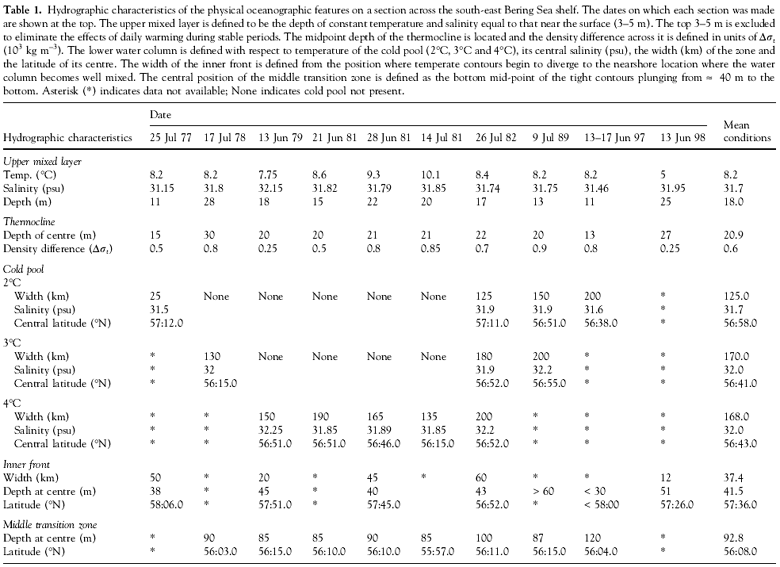
Table 1. Hydrographic characteristics of the physical oceanographic
features on a section across the south-east Bering Sea shelf. The dates on which
each section was made are shown at the top. The upper mixed layer is defined
to be the depth of constant temperature and salinity equal to that near the
surface (3-5 m). The top 3-5 m is excluded to eliminate the effects of daily
warming during stable periods. The midpoint depth of the thermocline is located
and the density difference across it is defined in units of 

 (103
kg m-3). The lower water column is defined with respect to temperature
of the cold pool (2°C, 3°C and 4°C), its central salinity (psu),
the width (km) of the zone and the latitude of its centre. The width of the
inner front is defined from the position where temperate contours begin to diverge
to the nearshore location where the water column becomes well mixed. The central
position of the middle transition zone is defined as the bottom mid-point of
the tight contours plunging from
(103
kg m-3). The lower water column is defined with respect to temperature
of the cold pool (2°C, 3°C and 4°C), its central salinity (psu),
the width (km) of the zone and the latitude of its centre. The width of the
inner front is defined from the position where temperate contours begin to diverge
to the nearshore location where the water column becomes well mixed. The central
position of the middle transition zone is defined as the bottom mid-point of
the tight contours plunging from  40 m to the bottom. Asterisk (*) indicates data not available;
None indicates cold pool not present.
40 m to the bottom. Asterisk (*) indicates data not available;
None indicates cold pool not present.
To illustrate the structure of the cold pool, the inner front and middle transition zone, we present observations from the transect occupied 26 July 1982 (Fig. 6a). This section was selected because the across-shelf structure on that day was closest to the mean conditions presented in Table 1. Moving seaward from the coastal domain where the water column is nearly isothermal (temperature difference from top to bottom is 0.1°C), the first feature encountered is the inner front. In this transect, the inner front forms a well-developed, sharp transition between middle shelf and coastal waters. The cold pool is well defined, with some horizontal variability in the temperature. At the seaward edge of the middle shelf, the isotherms become more tightly spaced horizontally, indicating the broad middle transition zone. Here, this increased horizontal temperature gradient extends from a depth of 40 m to the bottom and is centered at a bottom depth of 100 m. As generally occurs (Coachman, 1986), there is no surface manifestation of the middle transition zone.
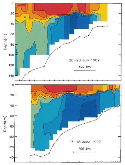
Figure 6. Contours of temperature (near the transect shown in Fig. 1) from CTD casts collected during (a, upper) July 1982 and (b, lower) June 1997. Cast locations are indicated by arrows at bottom of each panel. Contour intervals are 0.5°C.
In contrast with the typical transect of 1982, the 1997 transect (Fig. 6b) shows marked differences including a shallower mixed layer, a stratified water column extending inshore to a depth of <35 m, the broadest inner front ever observed, and a cold pool with the greatest horizontal extent. It should be noted that the 1997 transect was taken 5-6 weeks earlier in the year than the 1982 data, and some of these comparisons may therefore be biased. The transect during June 1998 was much shorter and is not shown, but strong contrasts between 1997 and 1998 are evident. During 1998, the water column was characterized by weak stratification over the middle shelf, an inner front centered about 130 km farther seaward than observed in 1997, and warmer bottom water (>3.5°C).
In the middle domain, the temperature structure of the water column from May
to October can usually be characterized by a top, mixed layer of warmer, fresher
water overlying a layer of colder, sometimes saltier water (the cold pool).
The two layers are separated by a thermocline, the thickness of which ranges
from <1 m to 15 m. The summer depth of the surface layer depends on wind
mixing; the bottom is tidally mixed. The integrated effect of wind, ice melt
and solar insolation determines the density difference ( of 0.25-1.25
in July) between the top and bottom layers of the water column.
There were marked differences in the temperature-salinity characteristics among the sampled years at Site 2 (Fig. 7). The large range in temperature usually makes it the dominant factor in determining the density structure, but during some years (most notably 1976, 1984, 1986 and 1997) salinity made a comparable contribution to density. During these four years, ice was present for at least several weeks, and the fresh water from the melting ice and weak winds stabilized the water column. During years when strong winds occur while sea ice is present or after its retreat, the low-salinity water from ice melt is mixed, reducing or removing the vertical salinity gradient. Strong vertical gradients in salinity are often associated with years when ice persists well into spring. The coldest bottom temperature occurred in 1976, the year with the most extensive ice cover on record; temperatures remained near freezing until late May. A strong density interface between the upper and lower layer (due both to temperature and salinity) inhibited the warming of the bottom layer, and thus enhanced the persistence of the cold pool. This occurred again in 1995, when the bottom layer was modified by the horizontal advection of cold saline water. In contrast, the density difference between the upper and lower layers in 1997 and 1998 was not particularly strong and thus permitted significant heating of the bottom layer.
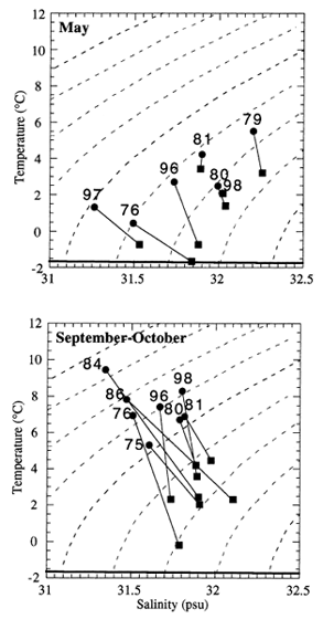
Figure 7. Temperature-salinity diagrams at Site 2 during (a, upper)
May and (b, lower) September/October. Lines of constant density are at intervals
of 0.25 . The
circles represent temperature and salinity at 5 m and the squares at 60 m.
Characteristics of middle shelf water temperature and salinity: Site 2
At two sites on the south-east Bering Sea shelf (Fig. 1), measurements of temperature, salinity, fluorescence and currents have been collected via moorings since 1995. From April through September, the ocean environment was monitored using surface moorings that also gathered meteorological data. During the rest of the year, because of the possible presence of sea ice, subsurface moorings were employed with the upper instruments at ~6 m below the surface. Details of the mooring design and instrumentation can be found in Stabeno et al. (1999).
The largest data set of oceanic variables has been collected at Site 2 in 70 m of water near the centre of the middle shelf (Fig. 1). From the examination of the transects along the hydrographic line discussed in the previous section, it is clear that this site is representative of a large portion of the south-eastern middle shelf. Temperature records from moorings (Fig. 8) reveal temporal variability on both seasonal and shorter time scales. In January, the water column is well mixed. This condition persists until buoyancy is introduced to the water column either through ice melt or solar heating. The very cold temperatures (shown in black in Fig. 8) that occurred in 1995, 1997 and 1998 resulted from the arrival and melting of sea ice. During 1996, ice was present for only a short time in February (when no mooring was in place). Generally, stratification develops during April. The water column exhibits a well-defined two-layer structure throughout the summer, consisting of a 15-25 m wind mixed layer and a 35-45 m tidally mixed bottom layer. Deepening of the mixed layer by strong winds and heat loss begins in August, and by early November the water column is again well mixed.
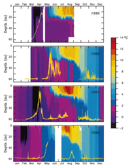
Figure 8. Temperatures measured at Site 2 (depth 70 m). Temperature was measured about every 3 m over the upper 30 m of the water column and then about every 5 m to the bottom. Each year there were three deployments of the instruments. Typically a subsurface mooring was deployed in September and recovered the following February. At this time two subsurface moorings are deployed. In April (after retreat of sea ice), a surface mooring is deployed and then recovered in September. The yellow line is fluorescence or chlorophyll at a depth of ~10 m. Each year the fluorescence is normalized to the maximum value of that year.
Using four years of mooring data, together with historical hydrographic data, we identified the timing and magnitude of the seasonal warming of the sea surface over the middle shelf (Fig. 9a). The upper layer begins to warm in early to mid-April, after the departure of any sea ice. Temperatures continue to increase to early August, when the maximum sea surface temperature typically occurs. During 1995-1998, the most rapid increase in near-surface temperature occurred in 1997 (~4.5°C month-1), while during the other three years warming was slower (~3.2°C month-1). In years before 1997, near-surface temperatures ranged from -1.7°C to 11.5°C, but temperatures well above this envelope were observed in the summer of 1997 and to a lesser extent in 1998. While the warmest near-surface temperature was observed in 1997, the water column as a whole was not particularly warm (Fig. 9b). The average water column temperature during 1997 was within the envelope of variability observed during the last 30 years. The warm surface temperatures that year were offset by a shallow mixed layer and cool bottom temperatures, so that the vertically averaged temperature was similar to that observed in 1995 and 1996. In contrast, the warm surface temperature of 1998 was complemented by the warmer-than-average bottom temperatures, resulting in the average temperature of the water column being the warmest in the last four years. The depth-averaged temperature in 1998, however, was still less than that observed in the warm years of the early 1980s.
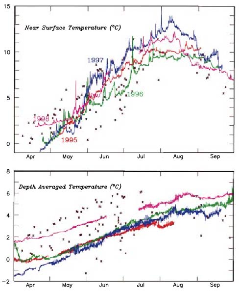
Figure 9. (a. upper) The seasonal signal of near-surface temperature at Site 2. Data from years when moorings were located at this site are indicated by coloured lines. Crosses represent data from hydrographic surveys between 1966 and 1994 collected within 25 km of Site 2. (b, lower) The depth-averaged temperature for the same data used in panel a.
During any given year, marked variations are superimposed on the spring-summer warming trend observed at Site 2 (Fig. 8). During 1995, ice persisted for more than a month; however, the water column was mixed to the bottom for only a short period in March. Advection of more saline water in the lower layer created a strong density gradient between the upper and lower layers (Stabeno et al., 1995). This effectively insulated the lower layer, limiting warming of the cold pool to less than 0.3°C month-1. The mixed layer was shallow (<20 m), because of the weak winds that summer (Fig. 3). During 1996, sea ice arrived early in February but remained for only a short time. Because strong winter winds mixed the water column after the ice departed, the density gradient was weak, and above-average wind mixing during the summer created a deeper surface layer than in 1995. Between April and August 1996, the bottom temperature warmed by about 1°C month-1. During 1997, ice was less persistent than in 1995; weak winds and strong heating resulted in a shallow, warm mixed layer. A storm in late May mixed the water column to 50 m, reducing the density gradient between the upper and lower layer. As in 1996, there was substantial warming (~1°C month-1) of the cold pool. In contrast to 1995 and 1997, ice arrived early in February 1998, during a period of weak winds. Thus, while the ice quickly cooled the upper layer, the lack of strong winds prevented mixing of fresh, cold water to the bottom. Only after the retreat of the ice in late February did wind energy become sufficient to mix the water column to the bottom. The mixing of the warm bottom water with the cold surface water produced above-average water column temperature for March. The water column then remained well mixed until late May. The weak stratification permitted a steady warming of the bottom layer by about 0.8°C month-1 from June to August.
In addition to temperature and salinity, fluorescence and chlorophyll were measured at the mooring sites. A phytoplankton bloom (indicated by fluorescence) occurred in March/April during 1995 and 1997, associated with the arrival and melting of sea ice (Fig. 8). The bloom began even though the water column was not stratified. In 1996 and 1998, when ice was present early in the year (January or February), the bloom occurred during May and appeared to last longer than observed in 1995 and 1997. During 1996 and 1998 the ice was present early in the year, when there was likely insufficient sunlight to initiate an ice-associated bloom.
While temperature data are more plentiful and define the seasonal cycle well, a significant part of the variability in density is due to salinity (Fig. 7). Using the same observations employed to delineate the envelope of variability of temperature at Site 2, we calculated the depth-averaged salinity there (Fig. 10a). The salinity in the vicinity of this location varies by almost 1.5 psu. The depth-averaged salinity was highest during 1966-1969 and 1977-1989. As already discussed, the years 1977-1989 had minimal ice coverage and thus less-than-average freshening due to ice melt. Historical records show that 1966 and 1967 were light ice years, while 1968 and 1969 were moderate (Overland and Pease, 1982). Salinity in 1995 was average (in spite of it being the most extensive ice year since 1976), but during 1996 and 1997 the water column was fresher. This was not solely due to freshening from melting sea ice, since both years had significantly less ice than 1995. There is evidence from satellite-tracked drifter tracks that during 1997 there was weaker-than-normal cross-shelf transport (not shown). Because the salinity of the water column near site 2 is a balance between the amount of ice melt (freshening) and the input of more saline water from the basin, a decrease in cross-shelf flux results in a fresher water column. The salinity of the water returned to a more moderate level in 1998, when there appears to have been enhanced cross-shelf transport.
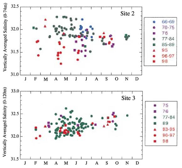
Figure 10. The depth-integrated salinity at Site 2 and at Site 3 from historical hydrographic casts. The casts from 1995 to 1998 are included. (a, upper) Measured near Site 2. (b, lower) Measured near Site 3.
Characteristics of outer shelf water temperature and salinity: Site 3
While not as extensive as the measurements at Site 2, data from Site 3 (at
water depth of 125 m over the outer shelf) provide insight into the response
of the outer shelf water to atmospheric, wind and ice forcing. Sea ice is less
common here than at Site 2. In the cold period (1972-1976), ice was present
for an average of 2-3 weeks a year, and during the warmer periods ice rarely
reached this location (Fig. 5). In only one of the mooring years (1995) was
ice blown over this site. During that year, a strong decrease in ocean temperature
was limited to a depth of 25 m, with weaker cooling occurring to ~80 m (Fig. 11).
Mean currents in this region are 5-10 cm s to the north-west (Stabeno
et al., 1999), so the cold water that results from the ice melt is
advected away. In 1997, ice extended into the vicinity of the mooring, although
it did not reach it. Remnants of the cold water from melting ice can be seen
in early April of that year (Fig. 11).
to the north-west (Stabeno
et al., 1999), so the cold water that results from the ice melt is
advected away. In 1997, ice extended into the vicinity of the mooring, although
it did not reach it. Remnants of the cold water from melting ice can be seen
in early April of that year (Fig. 11).
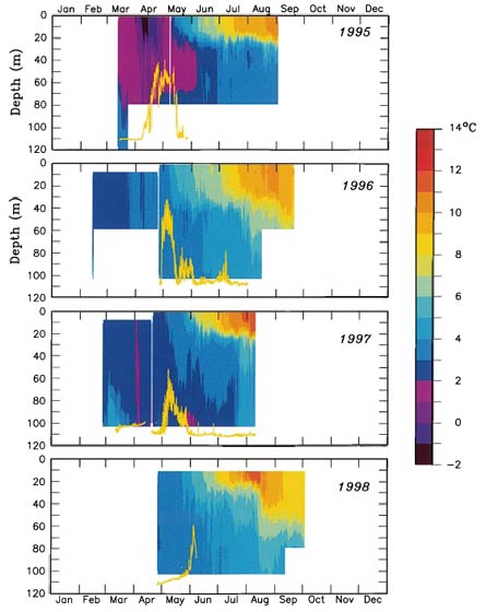
Figure 11. Temperatures measured at Site 3 (depth 125 m). Temperature
was measured every ~3 m in the upper 30 m and every 10 m below that. During 1995-1997, two moorings were
deployed in each year; during 1998, only a single mooring was deployed. The
yellow line is fluorescence or chlorophyll at a depth of ~10 m. Each year the
fluorescence is normalized to the maximum value of that year.
During the winter of most years, the water column at Site 3 was weakly stratified. Stratification owing to solar heating begins in May, with maximum temperatures occurring in late August. The depth of the mixed layer is similar to that observed at Site 2, but there is a greater transfer of heat below the upper mixed layer as a result of weaker stratification. The lack of moorings in autumn and early winter prevents us from describing the cooling of the water column. As at Site 2, the presence of ice can trigger an early spring bloom (1995). The spring bloom in 1996 and 1997 began in early May; in comparison, in 1998 it was delayed until late May by the strong mixing. In 1996 the bloom started at the same time at Site 2 and Site 3, but during 1998 the bloom at Site 3 appeared to be delayed by several weeks. In 1997, the bloom at Site 3 was much later than the ice-initiated bloom at Site 2.
Because ice is less common at Site 3, the major influence on salinity is cross-shelf advection. The variability of the depth-averaged salinity is less at Site 3 than at Site 2, and the marked freshening of the water column observed at Site 2 in 1996 and 1997 is not evident (Fig. 10b). There does appear to be a significant annual cycle at Site 3, with a systematic increase in salinity from spring until autumn. This increase is most pronounced in the lower part of the water column; salinity of the upper layer does not systematically change with the seasons. Unfortunately, there are no data taken during November-January when there must be a comparable decrease in salinity. This seasonal signal must result from variations in the onshelf flux of more saline water from the slope. The mechanism causing the annual cycle in salinity is not known, although instability in current along slope can result in onshelf flux (Stabeno and van Meurs, 1999).
Currents can be divided into high-frequency tidal currents and lower-frequency
flows. Most of the horizontal kinetic energy over the south-eastern shelf is
in the tidal currents; they play an important role in mixing and generation
of subtidal flow owing to their non-linear interaction with topographic features
(Stabeno
et al., 1999). Over the south-east shelf the dominant tidal constituent
is M , which has an amplitude of
~24 cm s at Site 2 and ~20 cm s
at Site 3. The dominant diurnal tide is K
, which has an amplitude of
~24 cm s at Site 2 and ~20 cm s
at Site 3. The dominant diurnal tide is K with tidal speeds about half of M.
In general, the annual mean flow is <5 cm s
towards the north-west, following bathymetry (Fig. 12). The strongest flow on
the shelf occurs at the shelf break and along the Alaskan Peninsula. The mean
flow in the centre of the shelf, near Site 2, is weak. Water from the western
Gulf of Alaska enters the shelf through Unimak Pass and continues to flow along
either the 50 m or 100 m isobath. This flow accounts for about one-third of
the flow through Bering Strait (0.35 × 10
with tidal speeds about half of M.
In general, the annual mean flow is <5 cm s
towards the north-west, following bathymetry (Fig. 12). The strongest flow on
the shelf occurs at the shelf break and along the Alaskan Peninsula. The mean
flow in the centre of the shelf, near Site 2, is weak. Water from the western
Gulf of Alaska enters the shelf through Unimak Pass and continues to flow along
either the 50 m or 100 m isobath. This flow accounts for about one-third of
the flow through Bering Strait (0.35 × 10 m3 s). The flow along the 100
m isobath is enhanced by flow up Bering and Pribilof Canyons, which also provide
on-shelf transport of nutrients and salt (Stabeno
et al., 1999). A weak cross-shelf flow north of the Pribilof Islands
transports nutrient-rich waters to the inner shelf region.
m3 s). The flow along the 100
m isobath is enhanced by flow up Bering and Pribilof Canyons, which also provide
on-shelf transport of nutrients and salt (Stabeno
et al., 1999). A weak cross-shelf flow north of the Pribilof Islands
transports nutrient-rich waters to the inner shelf region.
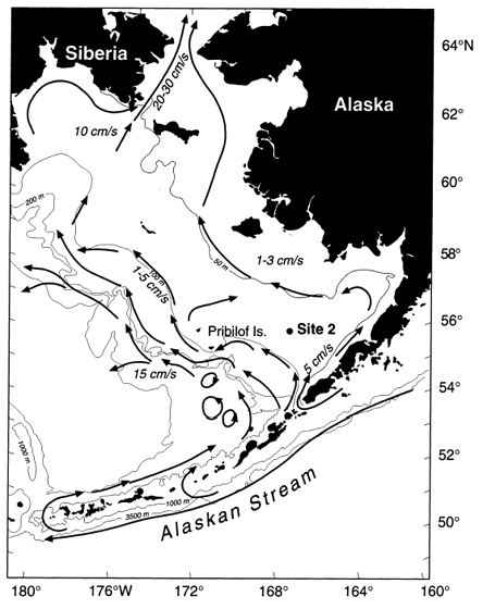
Figure 12. A schematic of flow on the eastern Bering Sea shelf in the upper 40 m of water column generated from a synthesis of moored current meters, satellite-tracked drift buoys and inferred geostrophic flow. Depths are in metres. (After Schumacher and Stabeno, 1998; Stabeno et al., 1999).
Long-term current measurements over the south-east Bering Sea shelf do not
exist, except for 34 months of noncontinuous current data at Site 2. The longest
continuous record was collected during 1996 with an acoustic Doppler current
profiler (ADCP) (Fig. 13). A 35-hour Lanczos squared filter was applied to each
of the time series to remove tidal and other high-frequency variability. Great
variations in direction and amplitude of the low-frequency currents are evident,
with stronger flow near the surface. These time series are representative of
all velocity records at this location. Statistics (Tables 2 and 3) provide the
mean monthly velocity and kinetic energy (calculated from these low-pass-filtered
data). Site 2 is in an area of weak mean currents, but currents averaged over
a shorter time scale (i.e. daily) can exceed 25 cm s. Throughout the year, the strongest flow occurred
in the upper water column, with weakest currents near the bottom. There was
a marked seasonal signal, with the most energetic currents occurring during
the winter and the weakest currents during the summer. The average velocity
over the 34 months of these records is 1.2 cm s to the west at a depth of 15 m and 0.2 cm s to the north-west at a depth of 60 m.
Figure 13. Time series of low-pass filtered currents as measured at Site 2 at (a) a depth of 14 m and (b) near the bottom at a depth of 68 m.
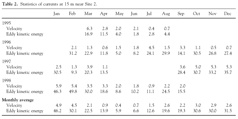
Table 2. Statistics of currents at 15 m near Site 2.
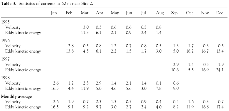
Table 3. Statistics of currents at 60 m near Site 2.
The strong winds during winter and spring 1998 forced stronger-than-average currents on the middle shelf. This flow during the winter likely resulted in strong cross-shelf transport of nutrients and salt, which would explain the observations of oceanic organisms along the Alaskan coast during May and the replenishment of salt at Site 2. In contrast, 1997 had particularly weak flows, as evidenced by the satellite-tracked drifting buoys that were deployed in the area during the spring and summer. Earlier research (Coachman, 1986) had concluded that because the mean flow over the middle shelf was weak, these currents would not play a role in replenishing nutrients and salt. Our ocean current records show that although annual and longer-term current velocities are weak, monthly mean currents can be persistent and can easily replenish nutrients and salt.
The Bering Sea shelf is a highly variable system at annual and interannual scales. The occurrence and melting of sea ice over the south-eastern shelf usually removes the previous year's heating. The combination of wind mixing and melting ice can cool the water column to about -1.7°C. This was seen in 1995 and 1997 but not in 1998, when weak winds during late winter were insufficient to mix the water column to the bottom at the time the ice was melting. Thus the bottom waters retained both heat and salt from the previous summer. Once mixing occurred after the retreat of the ice, the water column was warmer and saltier than 1995-1997.
The timing and extent of ice is crucial to determine the timing and rapidity of the phytoplankton bloom that occurs over the shelf in the spring. A climate shift that would decrease the extent of ice would have extreme effects not only on the water column structure but also on the phytoplankton blooms and the higher trophic levels that consume them.
Much of the eastern Pacific Ocean exhibited warm sea surface temperature (SST) anomalies during 1997. The SST anomaly extended northward from the Equator, where El Niño conditions existed, into the Arctic Ocean. The warming in the Bering Sea and Arctic Ocean is a consequence of local forcing rather than propagation of warm water from the Equator. In addition, changes in atmospheric forcing influenced the exchange with adjacent oceans (North Pacific and Arctic Oceans) and the circulation on both the Bering Sea basin and shelf. This has important repercussions for the Arctic Ocean. In 1998, warm water was noticed in the Arctic Ocean, which contributed to a reduction in the thickness and extent of the polar ice. The water in the Bering Sea likely enhanced this warming, because of the net northward flow through Bering Strait. Continued warm temperatures in the Bering Sea could have a significant impact on the Arctic ecosystem.
Two of the striking features of atmospheric forcing during 1997 and 1998 were a change in the timing of the last winter storm and weakening of summer (June-July) winds (Fig. 14). The Bering Sea ecosystem is particularly sensitive to storms during May (Sambrotto et al., 1986). The spring bloom strips the nutrients from the upper layer, and the stability of the water column isolates the nutrients in the lower layer. Thus storms in mid-to-late May provide important nutrients for continuation of blooms into summer, and lessen the density difference between the upper and lower layers, thus permitting subsequent minor mixing events to supply nutrients into the photic zone. Storms are less effective at entraining nutrients into the upper layer during June and July, both because they are weaker and because the seasonal strengthening of the thermocline inhibits mixing. From 1986 to 1996 the weather during May was particularly calm; in contrast, May in 1997 and 1998 was characterized by strong individual wind events, which weakened the stability of the water column, creating a pathway for greater nutrient supply, which prolonged primary production. In contrast to stronger winds in May, the summers of 1997 and 1998 had among the weakest mean wind stress since measurements began at St. Paul. This allowed for a shallow mixed layer and thus higher sea surface temperatures. If the pattern of late spring storms and weak summer winds persists, it could change the phytoplankton community. If primary production is prolonged into summer, the total productivity of the shelf could be enhanced, thus affecting higher trophic levels.
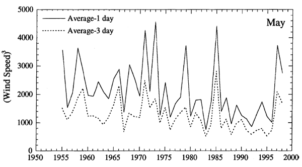
Figure 14. Maximum daily wind speed cubed (unbroken line) and 3 day average wind speed cubed (broken line) during May of each year. Winds were measured at St Paul Island.
Whether part of a long-period cycle or a persistent positive trend, the climate of the Arctic (including the Bering Sea) is warming. One example of this is the long-term warming trend in the atmosphere (0.75°C per decade) that occurred from 1961 to 1990 (Chapman and Walsh, 1993). The extent of the permafrost in the land masses surrounding the Bering Sea has decreased (Osterkamp, 1994) and the extent of many Alaskan glaciers has been reduced. A group of scientists convened in 1995 to hypothesize physical changes in the Bering Sea under a global warming scenario (US GLOBEC, 1996). Among the changes they forecast were that wind mixing energy, the supply of nutrients and ice extent/thickness would decrease and sea surface temperature would increase. This combination of conditions was observed during 1997 and may represent a foretaste of what will become typical in the future.
The implication of these changes in the physical environment to changes in biota is difficult to forecast, owing both to the complexity of the interrelationships and to the limited duration and spatial coverage of observations made in the Bering Sea. We need to continue monitoring this system to identify the mechanisms linking short- and long-term physical changes to ecosystem variability. With a better understanding of how the Bering Sea functions, human activities can be managed to minimize their impact on this ecosystem.
We thank Bill Parker, Carol Dewitt, David Kachel and Lynn Long for technical support, Richard Davis for processing of fluorescence data, and George Hunt for enthusiasm and leadership of the Inner Front Program. We express our thanks to the officers and crew of the NOAA Ships Miller Freeman, the R/V Wecoma, R/V Alpha Helix and the CCGS Sir Wilfred Laurier for their field support during the field work. This work was supported by NOAA's Coastal Ocean Program and by OAR, and by the National Science Foundation through the Inner Front Program. This is contribution FOCI-B352 to Fisheries Oceanography Coordinated Investigations, contribution 2040 to PMEL and contribution 657 to JISAO.
Baduini, C.L., Hyrenbach, K.D., Coyle, K.O., Pinchuk, A., Mendenhall, V., Hunt, G.L., (JR) (2001) Mass mortality of short-tailed shearwaters in the Eastern Bering Sea during summer 1997. Fish. Oceanogr. 10:117-130.
Barnston, A.G. and Livezey, R.E. (1987) Classification of seasonality and persistence of low-frequency atmospheric circulation patterns. Mon. Wea. Rev. 115:1083-1126.
Brodeur, R.D., Mills, C.E., Overland, J.E. and Schumacher, J.D. (1999) Massive increase in jellyfish biomass in the Bering Sea: possible links to climate change. Fish. Oceanogr. 8:296-306.
Chapman, W.L. and Walsh, J.E. (1993) Recent variations of sea ice and air temperatures in high latitudes. Bull. Am. Meteor. Soc. 74:33-47.
Coachman, L.K. (1986) Circulation, water masses, and fluxes on the southeastern Bering Sea shelf. Cont. Shelf Res. 5:23-108.
Francis, R.C., Hare, S.R., Hollowed, A.B. and Wooster, W.S. (1998) Effects of interdecadal climate variability on the oceanic ecosystems of the NE Pacific. Fish. Oceanogr. 7:11-21.
Horel, J.D. and Wallace, J.M. (1981) Planetary-scale atmospheric phenomena associated with the Southern Oscillation. Mon. Wea. Rev. 109:813-829.
Mantua, N.J., Hare, S.R., Zhang, Y., Wallace, J.M. and Francis, R.C. (1997) A Pacific interdecadal oscillation with impacts on salmon production. Bull. Am. Meteor. Soc. 78:1069-1079.
Miller, A.J., Cayan, D.R., Barnett, T.P., Graham, N.E. and Oberhuber, J.M. (1994) Interdecadal variability of the Pacific Ocean: model response to observed heat flux and wind stress anomalies. Clim. Dyn. 9:287-302.
Napp, J.M. and Hunt, G.L. Jr (2001) Anomalous conditions in the southeastern Bering Sea, 1997: linkages among climate, weather, ocean, and biology. Fish. Oceanogr. 10:61-68.
Napp, J.M., Kendall, A.W. Jr and Schumacher, J. D. (2000) A synthesis of biological and physical processes affecting the feeding environment of larval wall eye pollock (theragra chalcogramma) in the Eastern Bering Sea. Fish. Oceanogr. 9:147-162.
National Research Council (1996) The Bering Sea Ecosystem: Report of the Committee on the Bering Sea Ecosystem. Washington, DC: National Academy Press: 324 pp.
Niebauer, H.J. and Day, R.H. (1989) Causes of interannual variability in the sea ice cover of the eastern Bering Sea. Geol. J. 18:45-59.
Niebauer, H.J., Alexander, V., Henrichs, S.M. (1995) A time-series study of the spring bloom at the Bering Sea ice-edge. I. Physical processes, chlorophyll, and nutrient chemistry. Continental Shelf Res. 15:1859-1877.
Niebauer, H.J., Alexander, V.A. and Hendricks, S. (1990) Physical and biological oceanographic interaction in the spring bloom at the Bering Sea marginal ice edge zone. J. Geophys. Res. 95:22,229-22,242.
Niebauer, H.J., Bond, N.A., Yakunin, L.P. and Plotnikov, V.V. (1999) An update on the climatology and sea ice of the Bering Sea. In: The Bering Sea: a Summary of Physical, Chemical and Biological Characteristics and a Synopsis of Research. T.R. Loughlin and K. Ohtani (ed). North Pacific Marine Science Organization, PICES, Alaska Sea Grant, pp. 29-60.
Ohtani, K. and Azumaya, T. (1995) Influence of interannual changes in ocean conditions on the abundance of walleye pollock (Theragra chalcogramma) in the eastern Bering Sea. In: Climate Change and Northern Fish Populations. R.J. Beamish (ed.). Can. Spec. Publ. Fish. Aquat. Sci. 121:87-95.
Osterkamp, T.E. (1994) Evidence for warming and thawing of discontinuous permafrost in Alaska. Eos Trans. Am. Geophys. Union 75:85.
Overland, J.E. and Pease, C.H. (1982) Cyclone climatology of the Bering Sea and its relation to sea ice extent. Mon. Wea. Rev. 110:5-13.
Overland, J.E., Bond, N.A. and Miletta, J. (2001) North Pacific atmospheric and SST anomalies in 1997: links to ENSO? Fish. Oceanogr. 10:69-80.
Sambrotto, R.N., Niebauer, H.J., Goering, J.J. and Iverson, R.L. (1986) Relationships among vertical mixing, nitrate uptake and phytoplankton growth during the spring bloom in southeastern Bering Sea. Cont. Shelf Res. 5:161-198.
Schumacher, J.D. and Alexander, V. (1999) Variability and influence of the physical environment to the ecosystem in the Bering Sea. In: The Bering Sea: a Summary of Physical, Chemical and Biological Characteristics and a Synopsis of Research. T.R. Loughlin and K. Ohtani (eds). North Pacific Marine Science Organization, PICES, Alaska Sea Grant Press, 147-160.
Schumacher, J.D. and Stabeno, P.J. (1998) Continental shelf of the Bering Sea. In: The Sea, Vol. XI. The Global Coastal Ocean: Regional Studies and Synthesis. A.R. Robinson and K.H. Brink (eds). New York: John Wiley, Inc., pp. 789-822.
Stabeno, P.J. (1998) The status of the Bering Sea in the first eight months of 1997. PICES Press 6(1):8-11.
Stabeno, P.J. and van Meurs, P. (1999) Evidence of episodic on-shelf flow in the southeastern Bering. J. Geophys. Res. 104:29,715-29,720.
Stabeno, P.J., Schumacher, J.D., Davis, R.F. and Napp, J.M. (1995) Under-ice observations of water column temperature, salinity and spring phytoplankton dynamics: Eastern Bering Sea shelf. J. Mar. Res. 56:239-255.
Stabeno, P.J., Schumacher, J.D. and Ohtani, K. (1999) Physical oceanography of the Bering Sea. In: The Bering Sea: a Summary of Physical, Chemical and Biological Characteristics and a Synopsis of Research. T.R. Loughlin and K. Ohtani (ed). North Pacific Marine Science Organization, PICES, Alaska Sea Grant Press, pp. 1-28.
Sugimoto, T. and Tadokoro, K. (1997) Interannual-interdecadal variations in zooplankton biomass, chlorophyll concentration and physical environment of the subarctic Pacific and Bering Sea. Fish. Oceanogr. 62:74-93.
Trenberth, K.E. (1990) Recent observed interdecadal climate changes in the Northern Hemisphere. Bull. Am. Meteor. Soc. 71:988-993.
Trenberth, K.E. and Hurrell, J.W. (1994) Decadal atmosphere-ocean variations in the Pacific. Clim. Dyn. 9:303-319.
Trenberth, K.E. and Hurrell, J.W. (1995) Decadal coupled atmospheric-ocean variations in the North Pacific Ocean. In: Climate Change and Northern Fish Populations. R.J. Beamish (ed.). Can. Spec. Publ. Fish. Aquat. Sci. 121:15-24.
US GLOBEC (1996) Report on Climate Change and Carrying Capacity of the North Pacific Ecosystem. Berkeley, CA: Scientific Steering Committee Coordination Office, Dept Integrative Biology, University of California Berkeley. GLOBEC Rep. No. 15, 95 pp.
Vance, T.C. et al. (1998) Aquamarine waters recorded for first time in eastern Bering Sea. Eos Trans. Am. Geophys. Union 79(10):121;126.
Wyllie-Echeverria, T. and Wooster, W.S. (1998) Year-to-year variations in Bering Sea ice cover and some consequences for fish distributions. Fish. Oceanogr. 7:159-170.
Return to Abstract