Observations
The observational program
During 1984 and 1985, 35 current meters and six pressure gauges (Aanderaa model RCM-4 and WLR-5 or TG-3) were deployed on nine taut-wire moorings in the western Gulf of Alaska (Fig. 1). The moorings were arranged in three sections; data was recorded at section 1 (moorings 1, 2 and 3) for 5 months (August 1984 to January 1985) and at sections 2 (moorings 4, 5 and 6) and 3 (moorings 6, 7 and 8) for 11 months (August 1984 to July 1985). Current meter depths and locations are shown in Fig. 2. Some instruments measured temperature and conductivity which were used to estimate salinity. The six bottom pressure gauges were located one at each end of a section. All gauges were mounted in a well on the anchor to avoid the effects of mooring motion.
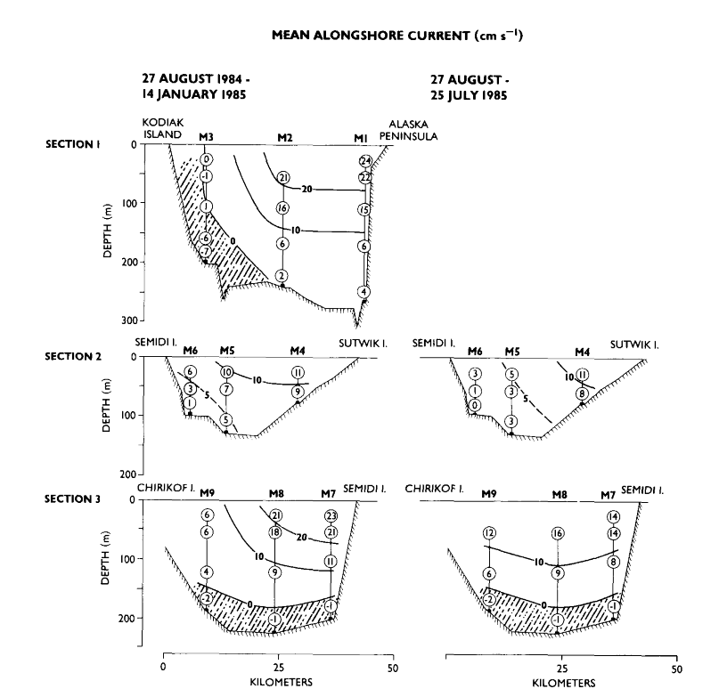
Figure 2. Mean current velocity observed at section 1 (top), section 2 (middle) and section 3 (bottom). Contours of the alongshore (220°T, 250°T and 190°T for sections 1, 2 and 3, respectively) component of velocity are shown in the left column for the period 27 August 1984 to 14 January 1985, and in the right column for the period 27 August 1984 to 25 July 1985. Shaded areas represent inflow.
Surface winds were computed from 6-hourly atmospheric surface pressure supplied by the Fleet Numerical Oceanography Center. These are geotriptic winds (a balance of Coriolis, pressure gradient, centrifugal and friction forces) which were rotated 15° counterclockwise, reduced in speed by 30% from the geostrophic wind, and interpolated to the vicinity of Semidi Islands (Fig. 3).
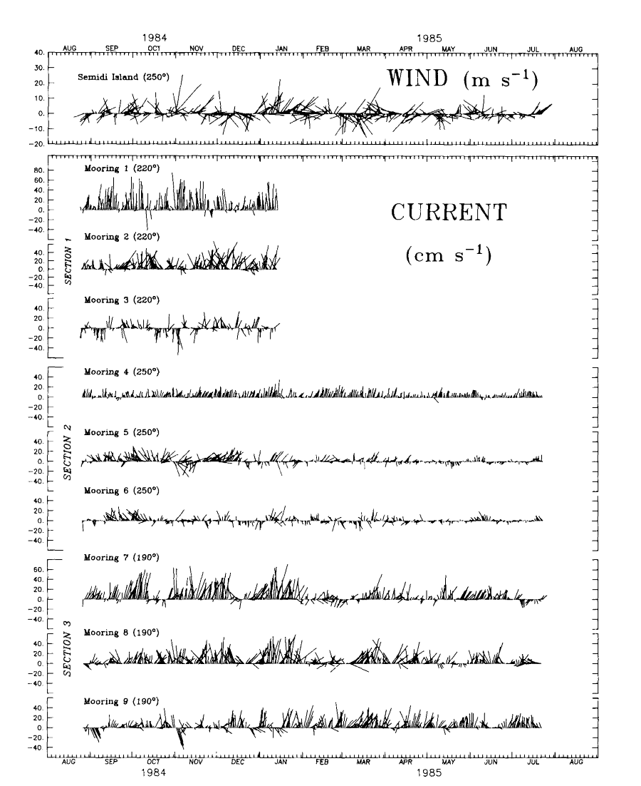
Figure 3. Current time series from a nominal depth of 56 m. The daily vectors are shown relative to the axis of each section (given in parentheses).
The data
Since tides dominated the bottom pressure spectrum, the pressure records were detided prior to low-pass filtering and removing linear trends. The current and detided bottom pressure data were low-pass filtered with a cosine-squared tapered Lanczos filter and resampled at 6-hourly intervals. This filter passes more than 99% of the amplitude at periods greater than 44 h, 50% at 35 h and less than 0.5% at 25 h, effectively removing the tidal signal from the current records. Examples of low-pass filtered currents are shown in Fig. 3.
Estimates of transport were calculated from the current velocity components normal to each section, multiplied by estimates of cross-sectional area. These areas were computed as follows. Detailed bathymetry was compiled for each section using information from continuous depth recordings, soundings at CTD stations and standard charts. Between moorings, the midpoint was used to define the horizontal extent assigned a given current velocity. The horizontal length between a mooring and the edge of a section varied. At section 1, current was assumed to occur only seaward of mooring 1 and to extend from mooring 3 to Kodiak Island. At section 2, the current was assumed to extend halfway between the outer two moorings and the adjacent land. At section 3, the current was taken to extend halfway between mooring 7 and Semidi Island but only one-third of the way (a depth of 100 m) to Chirikof Island. The vertical length at each mooring was selected as the midpoint between adjacent current meters. For example, the velocity from instruments at a nominal depth of 26 m (the next current meter was at 56 m) was assigned to the upper 41 m of the water column. We assumed no shear in current velocity within a transport layer. Velocity was set at zero approximately 5 m above the bottom. All results presented here are based on 6-hourly time series.
Mean and low-frequency transport. The structure of
the mean alongshore current shows the local manifestation of the ACC. During
the period August to January (Fig. 2, left
column), the ACC was strongest (>20 cm s )
in the upper 150 m on the northwest or west side of the sea valley at sections
1 and 3. The portion of the ACC which continued along the Peninsula (section
2), rather than following the sea valley (section 3), shows more moderate
(~10 cm s) flow. Inflow occurred in
both sea valley sections (1 and 3). When averages over the entire observation
period (August 1984 to July 1985: Fig. 2,
right column) are considered, the flow pattern at section 3 is changed substantially
from the August to January mean. Maximum velocities were smaller and more
evenly distributed across the sea valley, although inflow remained on the
bottom. This inflow supports conclusions from hydrographic data that an
"estuarine-like" or two-layered flow exits (Reed
et al., 1987) and emphasizes the care required in selecting a
level of no motion for baroclinic calculations (Reed
and Schumacher, 1989).
)
in the upper 150 m on the northwest or west side of the sea valley at sections
1 and 3. The portion of the ACC which continued along the Peninsula (section
2), rather than following the sea valley (section 3), shows more moderate
(~10 cm s) flow. Inflow occurred in
both sea valley sections (1 and 3). When averages over the entire observation
period (August 1984 to July 1985: Fig. 2,
right column) are considered, the flow pattern at section 3 is changed substantially
from the August to January mean. Maximum velocities were smaller and more
evenly distributed across the sea valley, although inflow remained on the
bottom. This inflow supports conclusions from hydrographic data that an
"estuarine-like" or two-layered flow exits (Reed
et al., 1987) and emphasizes the care required in selecting a
level of no motion for baroclinic calculations (Reed
and Schumacher, 1989).
From August 1984 to January 1985 the mean and r.m.s. error
of the volume flux through section 1 (
 )
was 0.81 ± 0.13 × 10
)
was 0.81 ± 0.13 × 10 m
m s and the sum of the transport through
the other two sections was 0.26 ± 0.04 (
s and the sum of the transport through
the other two sections was 0.26 ± 0.04 ( )
+ 0.68 ± 0.11 (
)
+ 0.68 ± 0.11 ( )
= 0.94 ± 0.13 × 10 m
s (
)
= 0.94 ± 0.13 × 10 m
s ( ).
During this interval, transport balanced to within 15%. For the longer time
interval (August 1984 to July 1985), mean volume transport in the ACC was
calculated to be 0.19 ± 0.02 ()
+ 0.66 ± 0.08 ()
= 0.85 ± 0.10 × 10 m
s ().
).
During this interval, transport balanced to within 15%. For the longer time
interval (August 1984 to July 1985), mean volume transport in the ACC was
calculated to be 0.19 ± 0.02 ()
+ 0.66 ± 0.08 ()
= 0.85 ± 0.10 × 10 m
s ().
Time series of transport through each of the three sections
and T are shown
in Fig. 4. The time series T
was formed by adding the 6-hourly low-pass filtered transport data from
sections 2 and 3; statistics were computed from this new series. All series
had high frequency (0.2-0.5 cpd) fluctuations which became less prominent
after May. These fluctuations were superimposed on a very low frequency
signal (~0.03 cpd) which also decreased in amplitude in spring. There were
four identifiable events in T
(Fig. 4, Table
1), each lasting more than 10 days, during which transport exceeded
the mean (0.85 × 10 m
s). To help visualize these events,
we applied a 10-day running mean to the transport series T.
The average duration of these events were 23 days with a standard deviation
of 11 days. During these pulses, the average transport was 1.49 × 10
m s.
The event with maximum transport occurred during January.
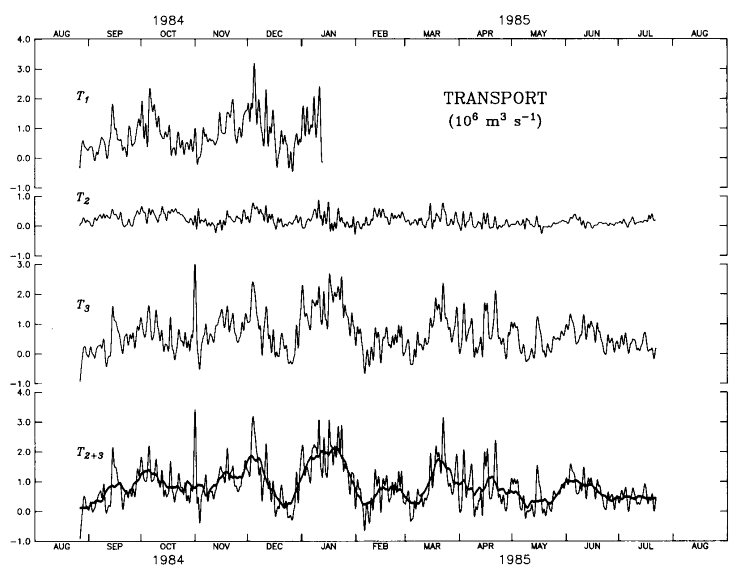
Figure 4. Time series of transport through sections 1,
2, 3 and the sum of T
+ T. (The heavy line
is a 10-day running mean.)
If your browser cannot view the following table correctly, click this link for a GIF image of Table 1.
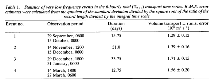
| Event no. | Observation period | Duration | Volume transport ± r.m.s error |
|---|---|---|---|
| (days) | 10 mł s |
||
| 1 | 29 September, 0600 | 15.75 | 1.29 ± 0.12 |
| 15 October, 0000 | |||
| 2 | 14 November, 1200 | 31.0 | 1.39 ± 0.16 |
| 15 December, 0600 | |||
| 3 | 29 December, 1800 | 33.75 | 1.71 ± 0.15 |
| 31 January, 0600 | |||
| 4 | 14 March, 1800 | 12.75 | 1.56 ± 0.20 |
| 27 March, 0600 | |||
Although the transport time series are rich in variability, spectral analysis showed no significant peaks (at the 95% significance level). For each series at least 66% of the variance occurred at periods longer than 10 days. The baroclinic instability identified in previous current data from Shelikof Strait was thought to be the source of most of the low-frequency current fluctuations (Mysak et al., 1981). This signal is clear in the current record from mooring 2 where the current vectors rotate back and forth across the section. Similar motion appears to a lesser degree at mooring 8. Analysis of current spectra, however, indicate that only at mooring 2 was the spectral peak statistically significant (Roach et al., 1987). In the time series of volume transport, baroclinic instability was not a mechanism generating significant variability.
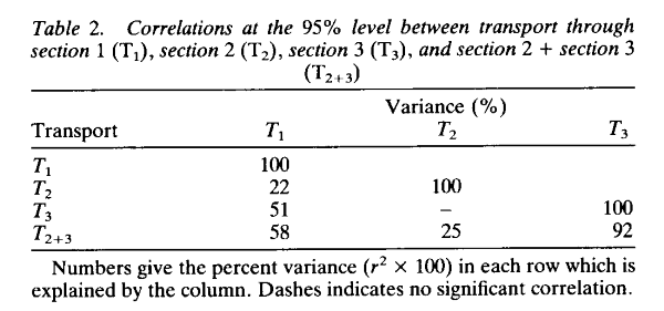
Relationships between transport time series. Fluctuations
in transport through sections 2 and 3 were best correlated with those upstream
through section 1 and were not significantly correlated with each other
(Table 2). Fluctuations
in T accounted for over
half of those in T.
For all pairs, most of the coherent signal was in the longest period band
(>19 days). Transports through sections 2 and 3 were coherent in only
one frequency band (4.6-5.1 days) and this accounted for less than 6% of
the total variance.
If your browser cannot view the following table correctly, click this link for a GIF image of Table 2.
| Variance (%) | |||
|---|---|---|---|
| Transport | T |
T |
T |
| T |
100 | ||
| T |
22 | 100 | |
| T |
51 | – | 100 |
T 
|
58 | 25 | 92 |
| Numbers give the percent variance
(r˛ × 100) in each row which is explained by the column. Dashes indicate no significant correlation. |
|||