U.S. Dept. of Commerce / NOAA / OAR / PMEL / Publications
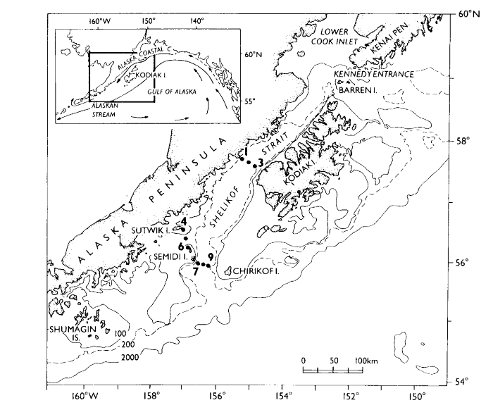
Figure 1. Study area setting. Positions of the nine moorings (dots) are indicated. Mooring numbers are consecutive but only outer ones are labeled. Shown in the insert is the regional circulation. Depths are in meters.
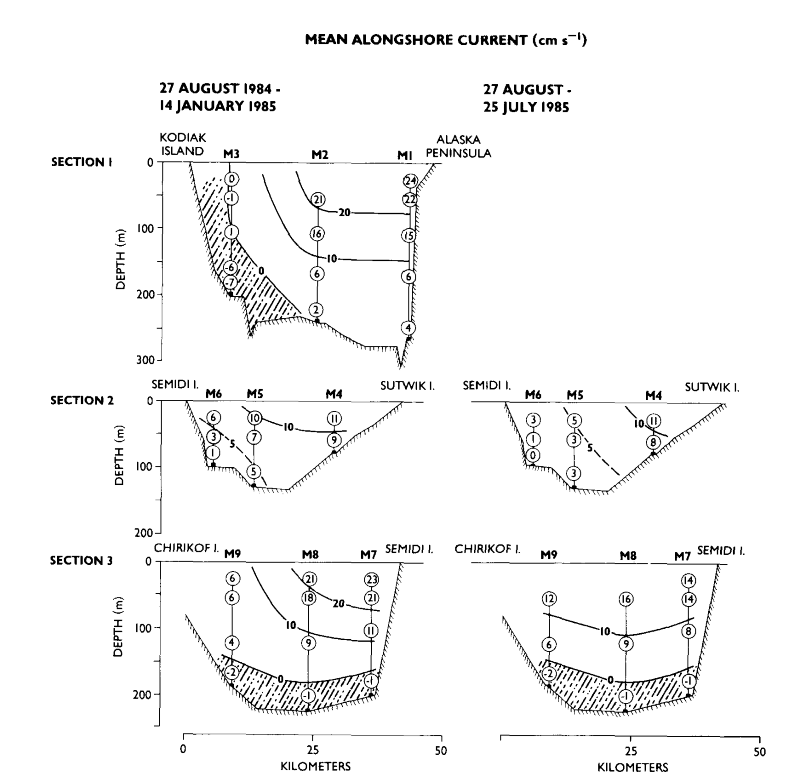
Figure 2. Mean current velocity observed at section 1 (top), section 2 (middle) and section 3 (bottom). Contours of the alongshore (220°T, 250°T and 190°T for sections 1, 2 and 3, respectively) component of velocity are shown in the left column for the period 27 August 1984 to 14 January 1985, and in the right column for the period 27 August 1984 to 25 July 1985. Shaded areas represent inflow.
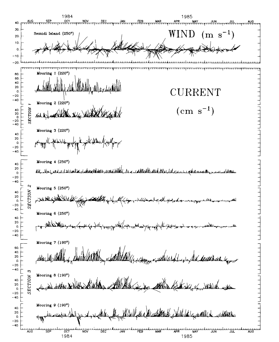
Figure 3. Current time series from a nominal depth of 56 m. The daily vectors are shown relative to the axis of each section (given in parentheses).
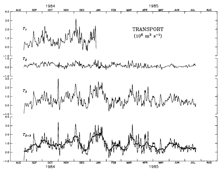
Figure 4. Time series of transport through sections 1, 2, 3 and the sum of T + T
+ T . (The heavy line is a 10-day running mean.)
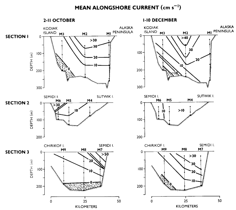
Figure 5. Structure of the mean current for (a) 2-11 October and (b) 1-10 December
1984. Volume transport at section 1 was 1.4 × 10 (1.7 ×
10), for section 2, 0.4 × 10 (0.5 × 10) and section 3,
1.0 × 10 (1.3 × 10) m
(1.7 ×
10), for section 2, 0.4 × 10 (0.5 × 10) and section 3,
1.0 × 10 (1.3 × 10) m s
s for the October
(December) event.
for the October
(December) event.
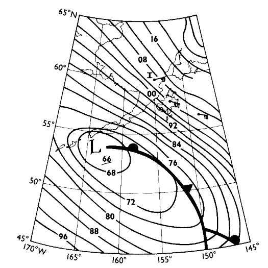
Figure 6. Sea level atmospheric pressure for 1200 on 31 October 1984. The wind barbs
are actual observations. Note how the barb at Iliamna (labeled I) indicates down-gradient
winds similar to those in Shelikof Strait. Surface wind at Semidi Island was 12.5 m s toward 300°T.
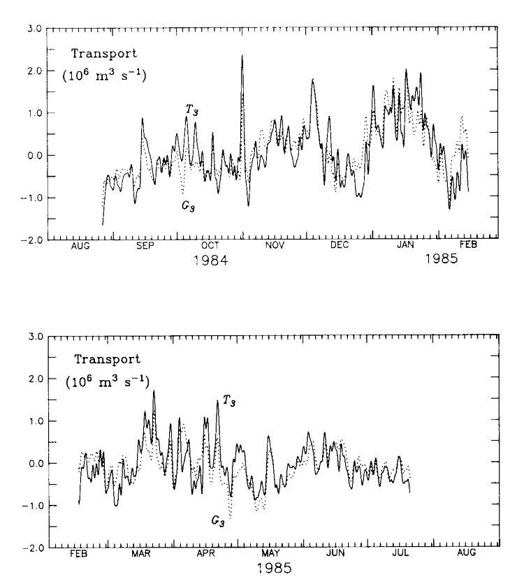
Figure 7. The demeaned and detrended time series of transport through section 3 from
current records (T, solid line) and
from the bottom pressure records from moorings 7 and 9 (G, dotted line).
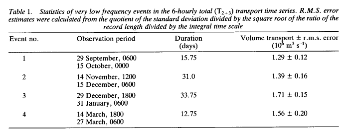
Table 1. Statistics of very low frequency events in the 6-hourly total (T ) transport time series. R.M.S. error
estimates were calculated from the quotient of the standard deviation divided by the
square root of the ratio of the record length divided by the integral time scale.
) transport time series. R.M.S. error
estimates were calculated from the quotient of the standard deviation divided by the
square root of the ratio of the record length divided by the integral time scale.
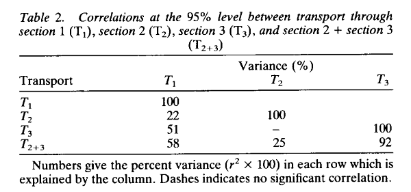
Table 2. Correlations at the 95% level between transport through section 1 (T ), section 2 (T), section 3 (T), and section 2 + section 3 (T).
Go back to References
Go to Abstract