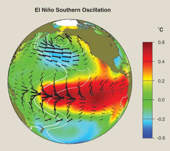
Fig. 1. El Niño anomalies in SST (color shading and scale in °C), surface atmospheric pressure (contours), and surface wind stress (vectors) in the Pacific basin. Pressure contour interval is 0.5 mb, with solid contours positive and dashed contours negative. Wind stress vectors indicate direction and intensity, with the longest vector equivalent to ~1 N m![]() . The patterns in this graphic are derived from a linear regression against SST anomalies averaged over 6°N–6°S, 90°W–180° in the eastern and central equatorial Pacific. All quantities scale up or down with the intensity of anomalies in this index region, that is, higher for strong El Niños and lower for weak El Niños. Anomalies of opposite sign apply to La Niña events, although there are some differences in the spatial patterns of El Niño and La Niña that this linear analysis does not capture [Larkin and Harrison, 2002; An and Jin, 2004].
. The patterns in this graphic are derived from a linear regression against SST anomalies averaged over 6°N–6°S, 90°W–180° in the eastern and central equatorial Pacific. All quantities scale up or down with the intensity of anomalies in this index region, that is, higher for strong El Niños and lower for weak El Niños. Anomalies of opposite sign apply to La Niña events, although there are some differences in the spatial patterns of El Niño and La Niña that this linear analysis does not capture [Larkin and Harrison, 2002; An and Jin, 2004].
Fig. 2. The Southern Oscillation index (SOI) and Niño-3.4 SST index for January 1950 to September 2006. This plot illustrates the coupled interactions between the ocean and the atmosphere that give rise to ENSO variations. Low SOI values are associated with weaker trade winds and warm sea temperatures (El Niño), whereas high SOI values are associated with stronger trade winds and cold sea temperatures (La Niña). The Niño-3.4 index is computed from monthly SST anomalies in the region 5°N–5°S, 120°–170°W. Positive anomalies >0.5°C indicate El Niño events, and negative anomalies 0.5 are shaded to emphasize the relationship with El Niño and La Niña. In the left panel, values have been smoothed with a 5-month running mean for clarity. The right panel shows the last 13 months of the record (unsmoothed) to highlight developing El Niño conditions in late 2006. Note the different scales for Niño-3.4 SST and SOI in the two panels.

Fig. 3. Statistical and dynamical model forecasts for SST in the Niño-3.4 region (5°N–5°S, 120°–170°W). Forecasts in most cases are from September 2006 initial conditions and are for seasonal averages from October-November-December (OND) 2006 through June-July-August (JJA) 2007 seasonal averages. Most models predict significant warm anomalies (>0.5°C anomaly), indicating the likelihood of a weak to moderate strength El Niño lasting at least into boreal spring 2007. The forecasts represent ensemble means or, for most statistical models, a single deterministic forecast. Institutions involved in issuing the forecasts are indicated by different symbols and listed at right (80). Area between the dashed lines at ±0.5°C indicates neutral conditions. Observed values (OBS) for July-August-September (JAS) 2006 and for September 2006 alone are shown as black diamonds. The inset shows observed SST anomalies averaged over 3 to 30 September 2006, with the Niño-3.4 region outlined. Contour interval in the inset is 0.5°C, with warm anomalies in yellow to red colors and cold anomalies in blue. See http://iri. columbia.edu/climate/ENSO/currentinfo/SST_table.html for a description of the various models and the methods by which the forecasts are compiled.
Return to Abstract