At the outset of TOGA the modeling and observational activities were relatively separate components of the program. However, as the program matured, a number of factors contributed to the development of a mutual dependency between TOGA models and observations. At a very basic level, data were needed for the development and validation of oceanic, atmospheric, and coupled models. Moreover, as experimental forecasts of ENSO became more routine and as initialization and assimilation techniques for coupled models took on greater importance, the modeling and observational components of TOGA developed a more intricate relationship. Overviews of the interaction between tropical models and data can be found in work by Latif et al. [this issue] and Stockdale et al. [this issue] and in the reviews by Knox and Anderson [1985], Philander [1990], and McCreary and Anderson [1991]. We concentrate here specifically on the evolution of this partnership toward improved model-based analyses and better coupled model initial conditions for predictions.
When considering the initialization of tropical ocean models and coupled prediction models, there are several factors that are critical. First, the tropical oceans are to a certain extent deterministic, by which we mean that adequate knowledge of past forcing in principle allows us to largely determine the state of the ocean. Knowledge of the surface wind stress is paramount in this determination. For example, Busalacchi and O'Brien [1980, 1981] demonstrated that, with a reduced gravity model and surface stress, one could capture key aspects of sea level variability associated with ENSO. Studies with ocean general circulation models (OGCMs) [e.g., Philander and Seigel, 1985; Harrison et al., 1990] also emphasized the paramount importance of wind forcing in model simulations. This fact makes the analysis and initialization problem quite different from that of numerical weather prediction, where there is no counterpart to the external forcing (and its associated errors) that are imposed through surface wind stress.
While in theory it is feasible that coupled tropical forecast models could be initialized with wind stress alone, practical considerations suggest that ocean thermal data will also be important. This is because wind stress and upper ocean thermal structure are partially redundant, so that observing and initializing baroclinic equatorial wave modes with subsurface temperature data could help correct some of the deficiencies in the imposed wind forcing. SST observations, either through assimilation or via surface boundary constraints, have also been important for the development of both the atmospheric and oceanic components of coupled prediction models. The ready availability, spatial coverage, and accuracy of SST analyses makes this variable particularly valuable for model validation and development [e.g., Stockdale et al., 1993].
From a historical perspective, sea level data has made one of the more significant contributions to ocean model development, particularly as equatorial theory was developing prior to TOGA. In situ sea level data continue to provide important model validation, particularly as sea level variations represent an integral, low baroclinic mode response to wind forcing and thermodynamic adjustments. With the advent of satellite altimetry, giving the spatial coverage not possible with in situ instrumentation, sea level may well assume far greater importance for model initialization.
Early studies in TOGA pointed to the advantages of thermal (mass) information vis-a-vis velocity information for ocean model initialization [Moore et al., 1987; Philander et al., 1987]. Hence, in a modeling context, velocity data have been used mostly for validation purposes [e.g., Leetmaa and Ji, 1989; Brady and Gent, 1994; Chen et al., 1994b; Fukumori, 1995; Halpern et al., 1995; World Climate Research Program, 1995a]. Various other data sets, such as those for salinity and surface heat fluxes, have also played important though somewhat less critical roles in model development. Consistent with these considerations and with the discussion in section 2.2 the National Research Council [1994a] ranked measurements in the following order of importance for the purpose of short-term climate prediction: (1) wind stress and SST, (2) subsurface thermal data, (3) sea level and ocean current data, and (4) salinity and atmospheric boundary layer data.
One of the focuses through the early part of TOGA was the assessment of the quality of various wind stress products. It was known that VOS winds would be useful but likely inadequate, but it was not immediately clear whether improved analysis techniques and improved numerical weather prediction schemes would make up for some of these inadequacies [e.g., Reynolds et al., 1989a]. Harrison et al. [1989] used a tropical ocean general circulation model to diagnose the impact of differences in various wind stress products. They compared simulations of the 1982-1983 El Niño forced by the Sadler and Kilonsky [1985] wind analysis (produced from VOS wind data and cloud drift winds), the FSU wind analysis [Goldenberg and O'Brien, 1981], and three analyses based on numerical weather prediction models (ECMWF, National Meteorological Center (NMC), and Fleet Numerical Oceanography Center (FNOC)). Overall, the research analyses [Goldenberg and O'Brien, 1981; Sadler and Kilonsky, 1985] produced more realistic dynamic responses but less convincing SST results for the equatorial waveguide. Simulations of the mean seasonal cycle and the 1982-1983 El Niño using linear dynamical ocean models [McPhaden et al., 1988b; Busalacchi et al., 1990] yielded similar results with regard to ocean dynamical responses, namely that the research products led to more realistic results. Details aside, one of the most important conclusions of these studies as far as TOGA was concerned was that improved knowledge of the surface wind stress was essential.
Operational atmospheric weather analysis and forecast models routinely merge observations of different parameters (e.g., temperature, winds, etc.) made at different levels in the atmosphere using different instruments. These analysis and forecast systems produce a dynamically consistent model atmosphere with high temporal and spatial resolution. For this reason the surface wind fields from such systems are often used to force ocean models like that run at NCEP for near-real-time tropical ocean analyses. Improving the quality of operational atmospheric model-based wind analyses is therefore an issue of some importance to climate modelers.
Operational centers now routinely use either wind speeds from the DMSP SSM/I instrument and/or vector winds from the ERS-1 and recently launched ERS-2 scatterometers. For example, the U.S. Navy [Phoebus and Goerss, 1991] and NCEP [Yu and Deaven, 1991] use the SSM/I wind speeds, while ECMWF [Gaffard and Roquet, 1995] and NCEP [Peters et al., 1994] use the ERS-1 and ERS-2 vector winds. The SSM/I winds are converted to vector winds using directions assigned from either the model forecast or a combination of the forecast and available data. Phoebus et al. [1994] reported that the greatest impact of the SSM/I was in the tropics and at higher latitudes along the meteorological storm tracks. Gaffard and Roquet [1995] found that the ERS-1 and ERS-2 vector winds improved the analyses in the southern hemisphere and had some positive impact in the short-range forecast.
TAO data are also used in operational weather forecast systems. Impact studies done at ECMWF, as reported by Anderson [1994], showed that differences between ECMWF analyses with and without TAO winds could exceed 3 m s-1, although typical differences were less. In addition, the impact of TAO observations tended to weaken significantly if the model was not reinforced with new TAO observations every 6 hours. Anderson [1994] pointed out that, in general, single level surface data like those from TAO buoys can be expected to have a relatively low impact on the atmospheric weather analyses. Reynolds et al. [1989a] reached a similar conclusion in a comparison of surface winds from the buoys with the winds from several different operational analyses. They found that the analyses looked more like each other than like the data. However, the models themselves have problems, as pointed out in a study by Williams et al. [1992]. They compared wind profile data at Christmas Island with the ECMWF forecast model and found that the model and the data were consistent above 1.5 km but not below this level. The model winds at these lower elevations were too weak and did not properly turn with height. This result suggests that there are problems in the model tropical boundary layer and that model and analysis systems need to be improved to optimize assimilation of tropical surface winds.
Recently, TAO and other TOGA-related data sets have been incorporated into atmosphere reanalyses at NCEP, ECMWF, and NASA Goddard Space Flight Center. These decade-long, internally consistent model analyses are produced using state-of-the-art numerical models, assimilation systems, and the most complete data sets available from historical archives [e.g., Schubert et al., 1993; Kalnay et al., 1996]. These analyses are valuable for providing initialization and validation fields for coupled model predictability studies, for determining the sensitivity of atmospheric models to slow variations in the surface boundary conditions, and for diagnostic studies of atmospheric variability. Evaluations of these reanalyses products are currently underway [e.g., Saha et al., 1995; Smull and McPhaden, 1996].
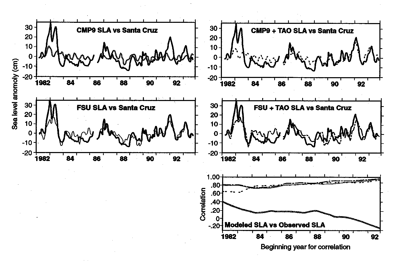
Availability of TAO data has led to efforts to develop improved surface wind analyses for ocean modeling through blending of buoy data with ship winds, satellite winds, and/or model output. Two studies illustrate this approach and the impact that TAO data make on such analyses. Menkes and Busalacchi [1995] performed a series of linear ocean model hindcasts for the equatorial Pacific using two baseline forcing functions over the period 1982–1993. The first, denoted CMP9, was based on winds derived from the NCEP medium-range forecast model as forced by observed SST but without incorporating any surface wind data or other meteorological data via an assimilation/analysis cycle. The other baseline wind product was the FSU winds. Beginning in November 1992, the FSU analyses incorporated TAO observations in increasing numbers (see Appendix B, section B1), but it is difficult to quantify the weight they were given in the subjective FSU analysis. Two combined data sets, CMP9 plus TAO and FSU plus TAO, were constructed by optimally interpolating the monthly TAO wind observations to each baseline forcing. Wind observations at each TAO location were converted to wind stress using the stability dependent parameterization of Liu et al. [1979]. Four sea level simulations were then performed and evaluated against tide gauge sea level measurements, gridded fields of TOPEX/POSEIDON sea level, and TOGA-TAO dynamic height anomalies across the equatorial Pacific Ocean.
The impact of TAO winds was characterized as a function of the increasing number of TAO observations with time. It was shown that the incorporation of a few TAO observations into the CMP9 wind product from 1987 onward compensated for the erroneously weak winds in the central and eastern equatorial Pacific and subsequently led to improved simulations (Figure 17). Similarly, the TAO observations also had a positive impact on the FSU simulation, both in terms of phase and amplitude, suggesting that the TAO observations be given greater weight in the FSU analysis. The impact of TAO observations in the 1990s, when the TAO array was reaching full deployment, was such that the improved simulations forced by FSU plus TAO and CMP9 plus TAO winds were quite similar, in contrast to earlier periods in the 1980s when the FSU and CMP9 simulations were very different.
Figure 17: Modeled sea level anomaly (SLA) versus observation at Santa Cruz, Galapagos Islands. (top left) CMP9 (dotted line) simulation versus observations (solid line). (top right) Same as Figure 17 (top left), but for CMP9 plus TAO (dashed line). (middle left) Same as Figure 17 (top left), with FSU (thin line). (middle right) Same as Figure 17 (top left), with FSU plus TAO (dot-dash line). (bottom) The correlation coefficient between the modeled and observed sea level anomalies as the time over which the correlation is computed progressively reduced by 1 year from its starting date (labeled on abscissa) to 1993. For example, the point labeled 1987 represents the cross correlation from 1987 through 1993.
A similar study was done by Reynolds et al. [1995] for the period April 1992 to April 1994. However, in this study they used the FSU product as well as two different monthly products: the lowest sigma level winds (roughly 40 m in height) from the NCEP operational medium-range forecast model with atmospheric data assimilation and ERS-1 wind stresses computed at a height of 10 m using the algorithm of Freilich and Dunbar [1993]. An objective analysis procedure [see Lorenc, 1981] was used to correct each of the wind fields with TAO data. Comparison of the corrections showed that all analyses tended to have zonal wind stresses that were too weak relative to TAO in the eastern tropical Pacific (Figure 18). Of the three wind products, however, the FSU analysis was in best agreement with TAO. NCEP stresses were too weak (i.e., consistently negative differences with TAO) during roughly the first half of the comparison period, although there appeared to be some improvement in the NCEP winds over the second half of the record. Conversely, the ERS-1 stresses were consistently too weak relative to TAO for the entire period.
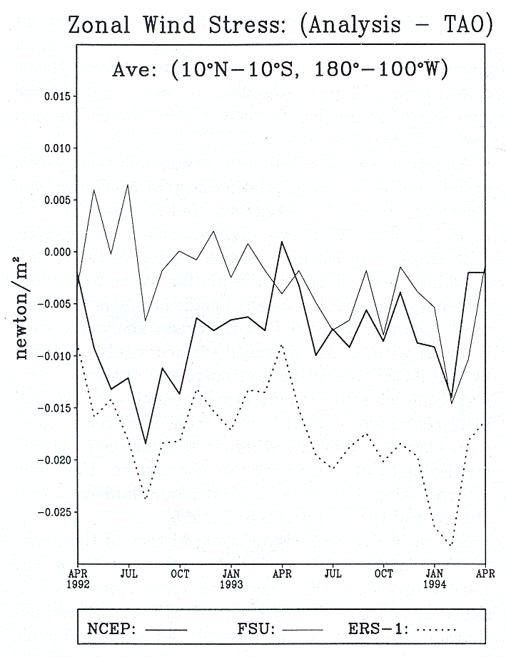
Figure 18: Zonal wind stress differences relative to TOGA-TAO for three products: NCEP, FSU, and ERS-1. The differences are averaged over 10°N to 10°S and 180° to 100°W. After Ji and Leetmaa [1997].
Reynolds et al. [1995] also used an ocean model to evaluate the impact of these different wind products. However, in contrast to Menkes and Busalacchi [1995], they used the general circulation model reported by Ji et al. [1995] both with and without the assimilation of thermal data. Results showed that assimilation was able to compensate for wind stress differences. Without assimilation, though, the ocean model was more affected by the different wind stress forcing. In particular, it was possible to clearly determine that ERS-1 zonal wind stresses were too weak in the eastern equatorial Pacific. However, the differences in the model fields compared to observations could not clearly identify which of the remaining three products (NCEP, FSU, and NCEP corrected by TAO) was superior. The Menkes and Busalacchi [1995] and Reynolds et al. [1995] studies differ because different wind stress fields and different models were used. However, in combination these studies indicate that TAO data have the strongest positive impact on the wind stress fields that are most independent of the mooring data.
Implementation of the TOGA observing system provided unprecedented opportunity for studying large-scale, low-frequency climate variability through the application of data assimilation techniques in combination with simple and complex tropical ocean models. Keys to achieving this were the vastly improved data coverage from the TOGA observing system, more effective data management strategies allowing rapid access to observations, order-of-magnitude improvements in computing capacity and resources, and improvements in ocean models.
Prior to TOGA, most oceanic observations were obtained from VOS lines, a handful of moorings and circulation drifters, and occasional research cruises. With the exception of SST, which could also be retrieved from satellite, it was essentially impossible to produce basin-scale ocean analyses from observations alone. With increased data coverage during TOGA, including a greatly enhanced volunteer observing ship network and the TAO array in the equatorial Pacific, regular and routine subsurface ocean analyses became possible. Several centers, including the El Niño Monitoring Center of the Japan Meteorological Agency (JMA), NCEP, the Joint Environmental Data Analysis Center in the United States, and the Bureau of Meteorology Research Center (BMRC) in Australia, began routinely producing monthly subsurface maps, particularly for the tropical Pacific.
All the data analysis and assimilation systems depend on knowledge of the amplitude and spatial and temporal scales of variability. Scale analyses, such as those of Meyers et al. [1991], Festa and Molinari [1992], and Kessler et al. [1996], provided estimates of signal levels versus unresolvable noise as well as estimates of the spatial and temporal covariance of the resolvable signal (which allow realistic scales for interpolation to be set). While the practical application of such information is not always straightforward, particularly when the first guess is provided by a dynamical model, it does nevertheless represent the fundamental basis for most of the applications described below.
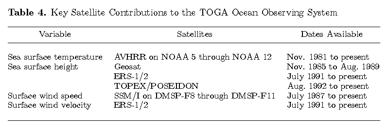
One example is the subsurface ocean analysis system developed at BMRC of Australia [Smith et al., 1991; Smith, 1995a]. This system uses optimal interpolation and a simple statistical forecast model to produce global upper ocean temperature analyses at periods from 10 days to 2 months, utilizing data from XBTs and TOGA-TAO. All quality control is objective [Smith, 1991] on the basis of information derived from the statistical interpolation. The shorter-period analyses were shown to retain all the important low-frequency, large-scale information of the bimonthly analyses (the analysis period upon which much of the TOGA observations were planned) as well as much of the interesting high-frequency fluctuations [Smith, 1995b]. Over monthly periods for the last half of TOGA, the estimated root-mean-square (rms) error variance in the 20°C isotherm analysis was typically 4–6 m (equivalent to around 0.3°C). Achieving such accuracy was a remarkable accomplishment, considering the low expectations for the measurement of subsurface thermal structure during TOGA as reflected in Table 4.
Dynamic ocean models have been used to simulate basin-scale ocean circulations long before TOGA. While such simulations did not usually ingest ocean information, they did represent an alternative route to ocean analyses, whereby information in the applied surface boundary forcing (principally the wind stress) was used to indirectly infer the state of the ocean. The main problems with model simulations were the poor quality of surface forcing, because of a lack of wind observations over the open ocean, and errors in the ocean model physical parameterizations. Limited in situ observations were primarily used for validation of model results. Although the quality of surface winds has improved steadily, especially since the TOGA observing system increased surface wind observations in the tropical Pacific, errors in the winds and in ocean models still significantly limit the accuracy of the simulations [Ji and Smith, 1995]. One way to compensate for errors in wind stress forcing and ocean model physics is to use data assimilation techniques to combine observations and model fields to yield the best possible estimate of the ocean state.
Data assimilation has been an active area of research from well before TOGA, although most practical applications were in the field of meteorology. Advances in ocean data collection, communication, and modeling in the late 1970s and early 1980s made ocean data assimilation a feasible option. Several studies have examined the problem of ingesting ocean subsurface data into simpler, linear, shallow water models of the tropical ocean [e.g., Moore, 1989, 1990, 1992; Moore et al., 1987; Moore and Anderson, 1989; Sheinbaum and Anderson, 1990a, b; Hao and Ghil, 1994; see also Busalacchi, 1996; Stockdale et al., this issue]. All these studies showed that subsurface sampling as practiced during TOGA could be used to correct model and wind-forcing errors and that the time taken for correction was only a month or so, owing to the rapid communication of information by equatorial waves.
An early attempt to produce routine ocean analyses utilizing an ocean data assimilation technique was a system developed by Leetmaa and Ji [1989] for the tropical Pacific. This system used wind-forced ocean model simulation as a first guess and combined the observations collected during a period of 1 month with the model field using the optimal interpolation. The data assimilation procedure was done monthly.
The main advantage to the model-based analyses is that large areas of data void are filled in by model dynamics. The main drawback to the sequential initialization method is that the data assimilation can introduce a strong shock when corrections are applied to the model fields, as discussed by Moore [1990]. Also, for models integrated forward in time until the next data assimilation cycle without continuous constraint by observations, model fields will drift toward the model's own equilibrium state. Hence a "sawtooth" pattern in the time history of the analyses is sometimes obvious [e.g., Hayes et al., 1989a].
A data assimilation system developed by Derber and Rosati [1989] was a significant improvement over earlier ocean analyses. This system is based on a variational method in which assimilation is done continuously during the model integration. Corrections to the model are spread over a long period of time; thus change to the model temperature field during each model time step is incremental. This significantly reduces the impact to the dynamical balances of the model fields and also keeps model fields from drifting toward their own climate. Further, an observation is retained in the model for a long period of time (2–4 weeks), weighted by the difference between the model time and the observation time during each assimilation time step. This procedure significantly increases the influence of observations to compensate for the lack of spatial and temporal data coverage in many areas. The drawback in doing this is that it tends to limit the analyses to resolving only large spatial scales and low-frequency phenomena [Halpern and Ji, 1993].
An operational model-based ocean analysis system based on the data assimilation system of Derber and Rosati [1989] has been implemented at the NCEP [Ji et al., 1995]. Real-time observations from satellite, VOS ships, and drifting and moored buoys are assimilated into an ocean general circulation model to produce near-real-time (weekly mean) Pacific and Atlantic analyses. The near-real-time NCEP ocean analysis system is forced with weekly averaged surface winds produced by the NCEP operational atmospheric analyses. Retrospective monthly Pacific Ocean reanalyses have also been generated at NCEP by forcing the ocean model with historical monthly wind-stress analyses produced at Florida State University [Stricherz et al., 1992] and incorporating additional delayed mode data not available in real time [Ji and Smith, 1995].
Shown in Figure 19 is the time history of the depth of 20°C isotherm anomalies along the equator in the Pacific for 1982–1995. The thermocline anomalies produced by the ocean analysis system (Figure 19, middle) showed variability in the central and western Pacific stronger than that produced by a model forced with the FSU winds without data assimilation (Figure 19, right). Comparisons with in situ observations of moorings and tide gauges suggest that the model-based analyses are of higher accuracy than the wind-forced simulation [Ji and Smith, 1995]. These studies show that even when using a high-quality wind stress forcing and a state-of-the-art ocean general circulation model, ocean data assimilation can still further improve the quality of analyses by compensating for errors in the forcing and model.
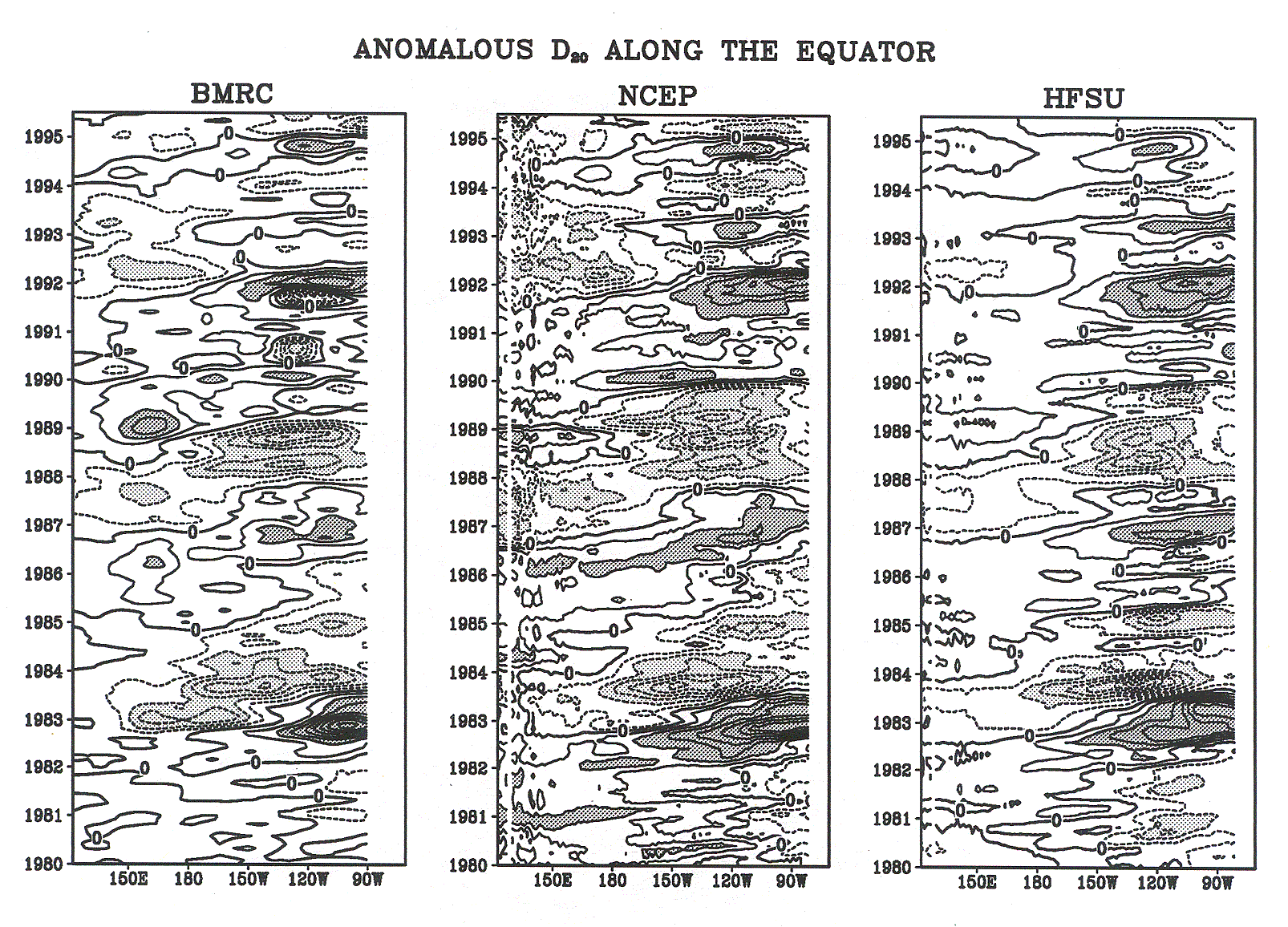
Figure 19: Anomalous depth of the 20° isotherm along the equator for the Pacific produced (left) by BMRC, (middle) by the NCEP ocean analysis system, and (right) by an ocean model simulation forced with monthly surface wind analyses from FSU. The contour interval is 10 m. Anomalies greater (less) than 20 m (-20 m) are indicated by dark (light) shading. From Ji and Leetmaa [1997].
Also shown in Figure 19 (left) are the 20°C isotherm depth anomalies from the BMRC subsurface analysis system, which is based on statistical analyses rather than dynamical model analyses [Smith, 1995b]. It should be noted that the NCEP and BMRC systems have quite different approaches to quality control (subjective versus objective) and to assimilation/inter- polation (continual insertion with variational con-straints versus sequential single-period optimal interpolation). The analyzed peaks and depressions of the thermocline depth from the NCEP and BMRC systems are generally similar (e.g., the peak anomalies of the 1982–1983 and 1991–1992 warm and 1984 cool events), as should be expected since they are essentially based on the same data sets. There are, however, some significant differences; the NCEP analysis of the 1984 cooling is characterized by a coherent west-to-east evolution, whereas the BMRC analysis shows essentially in-place cooling. Such differences reflect the different modes of interpolation; the dynamic system has theoretical advantages for transferring information within the equatorial waveguide but at the same time may be hampered by errors in the wind and/or the model.
A promising way of improving tropical ocean model-based analyses is through the assimilation of altimetry data [see, e.g., Arnault and Perigaud, 1992]. This requires projection of sea level variability onto baroclinic ocean thermal structure, which can be readily done by developing empirical relationships between the two variables [e.g., Rebert et al., 1985; Carton et al., 1996]. Advanced techniques such as the Kalman filter and the adjoint method have been used to assimilate Geosat and TOPEX/POSEIDON altimetry data into simple reduced-gravity models [e.g., Gourdeau et al., 1997; Greiner and Perigaud, 1994, 1996; Fu et al., 1993; Fukumori, 1995]. Impact studies of altimetry assimilation on ocean general circulation model-based analyses have also been performed Carton et al. [1996], and Fischer et al., 1997].
Assimilation of observations obtained from the TOGA observing system not only provides means to produce much improved ocean analyses, it also provides a great opportunity for improving the definition of the initial ocean fields for prediction of ENSO using coupled models. This is discussed in section 4.4. Analyses such as those described above have also found a wide range of other applications. For example, Lukas et al. [1995] studied the large-scale variations of the Pacific Ocean during TOGA COARE using the NCEP subsurface analyses, providing a context for the analysis of observations of air-sea interaction in the intensive flux array. The use of model-based analyses for process studies is now quite common in meteorology, and the advances in ocean analysis and assimilation during TOGA will assist in making such applications more common in climate studies.
Finally, analysis systems have been used to examine the design of the TOGA subsurface observing system. Miller [1990] investigated the impact that ocean thermal data (processed to estimates of dynamic height) might have in hindcasts of sea level in the equatorial Pacific. His results suggested that the TAO array would positively impact on hindcasts of monthly mean sea level. Smith and Meyers [1996] have examined the relative impact of XBT and TOGA-TAO data for monitoring tropical Pacific Ocean thermal variability. They concluded that for the last half of the TOGA period, over the region 20°S–20°N, the net information content of the systems were comparable in magnitude, each contributing the equivalent of around 300 independent subsurface samples per month.
ENSO prediction depends strongly on the accuracy of the ocean initial conditions. Three different methods are presently used for initialization of the ocean for ENSO predictions using coupled ocean-atmosphere models. The first method, used by Cane et al. [1986], is to spin up the ocean using the observed surface wind history prior to the initiation of a forecast. A second method uses assimilation of subsurface temperature data together with surface wind forcing to achieve better defined subsurface ocean states. This is done at the NCEP [Ji et al., 1994] and at the Geophysical Fluid Dynamics Laboratory (GFDL) [Rosati et al., 1997]. A third method developed at BMRC utilizes both wind and subsurface data jointly to initialize a coupled model through an adjoint data assimilation method [Kleeman et al., 1995].
Assimilation experiments described in the previous section illustrated the need to assimilate data in such a way that initialization "shock" is minimized. On the other hand, these studies demonstrated the potential impact of data assimilation on the forecast of eastern equatorial Pacific SSTs several seasons into the future. Ji and Leetmaa [1997], for example, compared results from forecast experiments initiated from ocean initial conditions produced with data assimilation and produced with wind forcing alone, using the NCEP coupled ocean-atmosphere forecast model [Ji et al., 1994]. Shown in Figure 20 are temporal anomaly correlation coefficients (ACC) and root-mean-square (rms) errors as a function of forecast lead times for area-averaged SST anomalies between forecasts and observations for an eastern equatorial Pacific region (120°–170°W, 5°S–5°N). The forecasts were initiated monthly for the period of 1983–1993. This comparison demonstrates convincingly that data assimilation has a significant positive impact on improving ENSO forecast skill. Ji and Leetmaa [1997] also showed forecast skills using ocean initial conditions produced with assimilation of XBT data alone and with assimilation of both XBT and TAO buoy data. The results indicate significant positive impact of the TAO buoy data, largely due to the vastly improved spatial and temporal data coverage by the TAO array in the tropical Pacific.
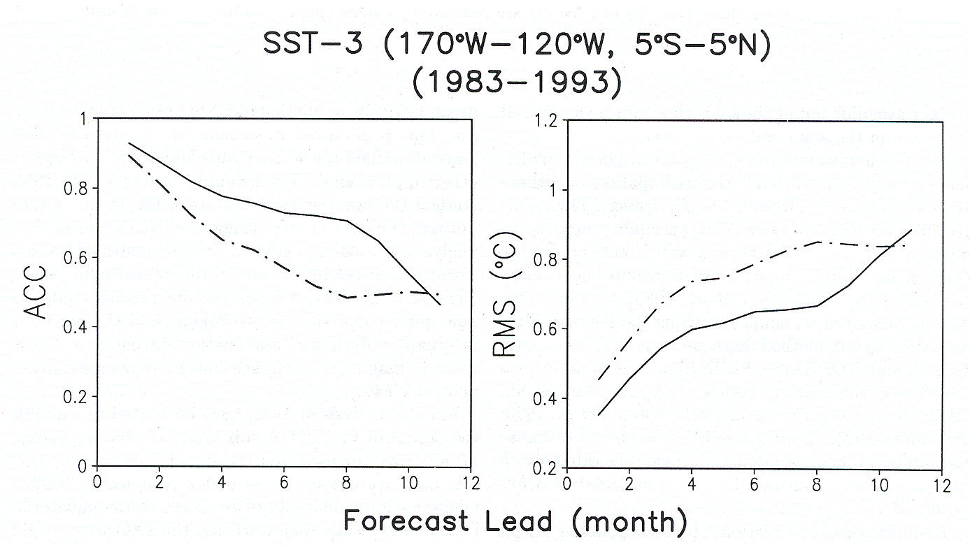
Figure 20: (left) Anomaly correlation coefficients and (right) rms errors between forecasts and observations for area-averaged SST anomalies in the eastern equatorial Pacific region between 170°–120°W and 5°S–5°N. Solid (dash-dot) lines are for forecasts initiated from ocean initial conditions produced with (without) subsurface data assimilation.
Kleeman et al. [1995] also demonstrated how enhanced forecast skill could be achieved in an intermediate coupled model by improving the initial conditions for upper ocean heat content. In this study the adjoint for the ocean component of the coupled model was used to improve the ocean initial conditions by finding a condition that was consistent with both the wind forcing and the subsurface ocean thermal data. Two sets of experiments were performed for the period January 1982 through October 1991. In the first experiment the ocean initial conditions were obtained by forcing the ocean model with the FSU winds. This initialization procedure was consistent with that of Cane et al. [1986], and similar forecast skill scores were obtained. In the second experiment improved initial conditions were obtained by using analyzed subsurface temperature anomalies averaged over the upper 400 m of the water column [Smith, 1995b] for the 12 months prior to initiating a coupled forecast. The use of the ocean data assimilation in this case led to notable increases in forecast skill.
Altimetry data, in addition to upper ocean thermal data, likewise have the potential for improving the skill of short-term climate predictions. [Fischer et al., 1997; M. Ji, R. W. Reynolds, and D. W. Behringer, Use of TOPEX/POSEIDON sea level data of ocean analyses and ENSO prediction: Some early results, submitted to the Journal of Climate, 1998]. In one set of experiments, for example, sea level data from TOPEX/POSEIDON were added to the XBT and TAO ocean model assimilation system of Ji et al. [1995]. The sea level data improved the agreement of the model sea level with independent tide gauge data and led to a more realistic forecast of tropical Pacific SSTs. On the other hand, predictability experiments using the Zebiak and Cane [1987] coupled model indicated that forecast errors were not reduced by using altimetry data for ocean model initialization [Cassou et al., 1996]. Thus, the utility of altimetry for initialization is model dependent, so that more research will be required to fully exploit altimetry for ENSO prediction.
In the previous initialization studies the oceanic component was first forced by observed wind stress and adjusted by assimilating subsurface thermal observations. Subsequently, the model-simulated SST was used to force the atmospheric component. However, a potential problem with this common approach is that since there are no interactions allowed between the oceanic and atmospheric components during initialization, the coupled system is not well balanced initially and may experience a shock when the forecast starts. Further, the imbalances between the mean states of the oceanic initial conditions and the coupled model contribute to systematic error of the forecast fields [Leetmaa and Ji, 1996]. In the study by Chen et al. [1995], initial conditions for the Cane and Zebiak [1985] model are generated in a self-consistent manner using a coupled data assimilation procedure. Initial conditions for each forecast are obtained by running the coupled model for the period from January 1964 up to the forecast starting time. At each time step prior to the forecast a simple data assimilation procedure is used whereby the coupled model wind stress anomalies are nudged toward the FSU wind stress observations. In this manner the coupled model itself is used to dynamically filter the initial conditions. Initialization shocks are reduced by providing a better balanced set of ocean-atmosphere initial conditions for the coupled forecast. Previously, the ocean initial conditions contained considerable high-frequency energy when forced by the FSU wind stress anomalies. The influence of the coupled model in the new initialization preferentially selects the low-frequency, interannual variability. This approach also results in a shallower thermocline in the western equatorial Pacific during most ENSO warm events with important implications for improved forecasts of warm event termination. Moreover, the coupled approach to initialization eliminates the springtime barrier to prediction that characterizes most coupled forecast schemes.
Recently, decadal-scale variability in the forecast skill has been noted in coupled models. Chen et al. [1995], for example, found that for the period 1982–1992, forecast skill was generally high for lead times of 12–24 months. Conversely, for the period 1972–1981, forecast skill was generally low for lead times longer than a few months. Balmaseda et al. [1995] also found generally higher predictability in the 1980s compared to the 1970s, and Goddard and Graham [1997] described reduced predictability associated with the 1993 and 1994–1995 El Niños relative to El Niños during 1982–1992. ENSO variations in the 1980s were generally stronger than those during the 1970s or during 1993–1995, suggesting that stronger ENSO events may be easier to predict than weaker events. It is also likely that the present generation of prediction models does not adequately represent the full range of physical processes responsible for the ENSO cycle or the interaction of ENSO with decadal time scale variations. These limitations could contribute to decadal fluctuations in predictability as well.
Although most data assimilation efforts in support of coupled models have focused on improving initial conditions, data assimilation techniques such as the Kalman filter have also been used as a means of parameter estimation in simple coupled models. In idealized versions of intermediate coupled models, there exist key parameters that govern the coupling strength between SST and the surface winds and the relation between the depth of the thermocline and the temperature of the water entrained into the ocean mixed layer. The particular values of these coefficients tend to determine the behavior of the coupled mode characteristic of the system. Similar to the way in which assimilation techniques have been used to estimate parameters such as the phase speed in shallow water models, the work of Hao and Ghil [1994] demonstrated how subsurface thermal data from the TAO array could be assimilated into coupled models to guide the proper estimation of key model parameters.
Return to previous section or go to next section