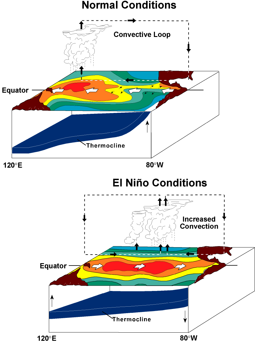
Figure 1: Schematic of normal and El Niño conditions in the equatorial Pacific. See section 2 for discussion.
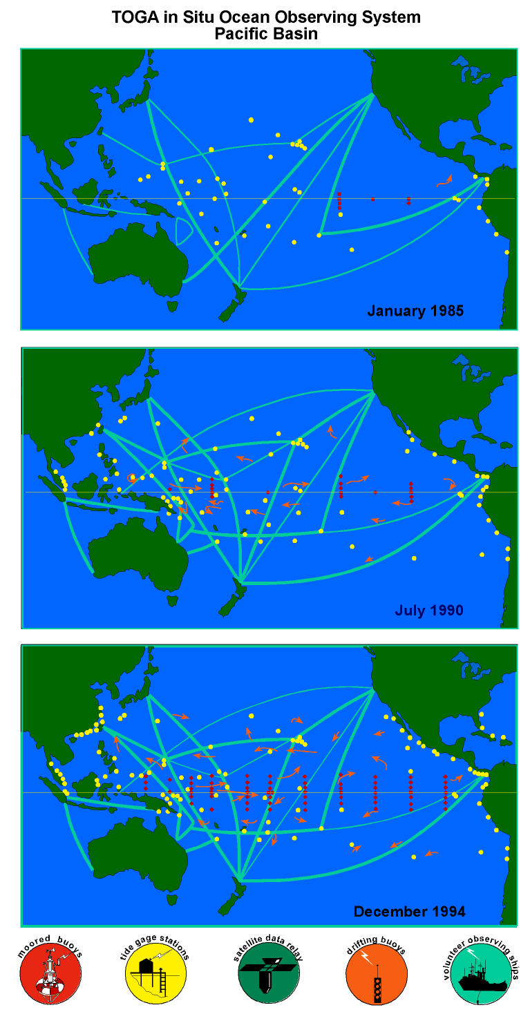
Figure 2: The in situ Tropical Pacific Ocean Observing System developed under the auspices of the TOGA program. (top) The observing system in January 1985 at the start of TOGA; (middle) the observing system in July 1990 at the time of the TOGA midlife conference in Honolulu [World Climate Research Program, 1990b]; (bottom) the observing system in December 1994 at the end of TOGA. The four major elements of this observing system are (1) a volunteer observing ship expendable bathythermograph program (shown by schematic ship tracks); (2) an island and coastal tide gauge network (circles); (3) a drifting buoy program (shown schematically by curved arrows); and (4) a moored buoy program consisting of wind and thermistor chain moorings (shown by diamonds) and current meter moorings (shown by squares). Thick ship tracks indicate expendable bathythermograph sampling with 11 or more transects per year; thin ship tracks indicate sampling with 6–10 transects per year. Although emphasis is on 30°N–30°S, termini of VOS XBT lines originating outside these limits are nonetheless shown. One drifting buoy schematic represents 10 actual drifters. Only those tide gauge stations are shown that reported their data to the TOGA Sea Level Center in Honolulu within 2 years of collection. Some tide gauge stations are so close as to be overplotted on one another. By December 1994 most measurements made as part of this four-element observing system were being reported in real time, with data relay via either geostationary or polar orbiting satellites.
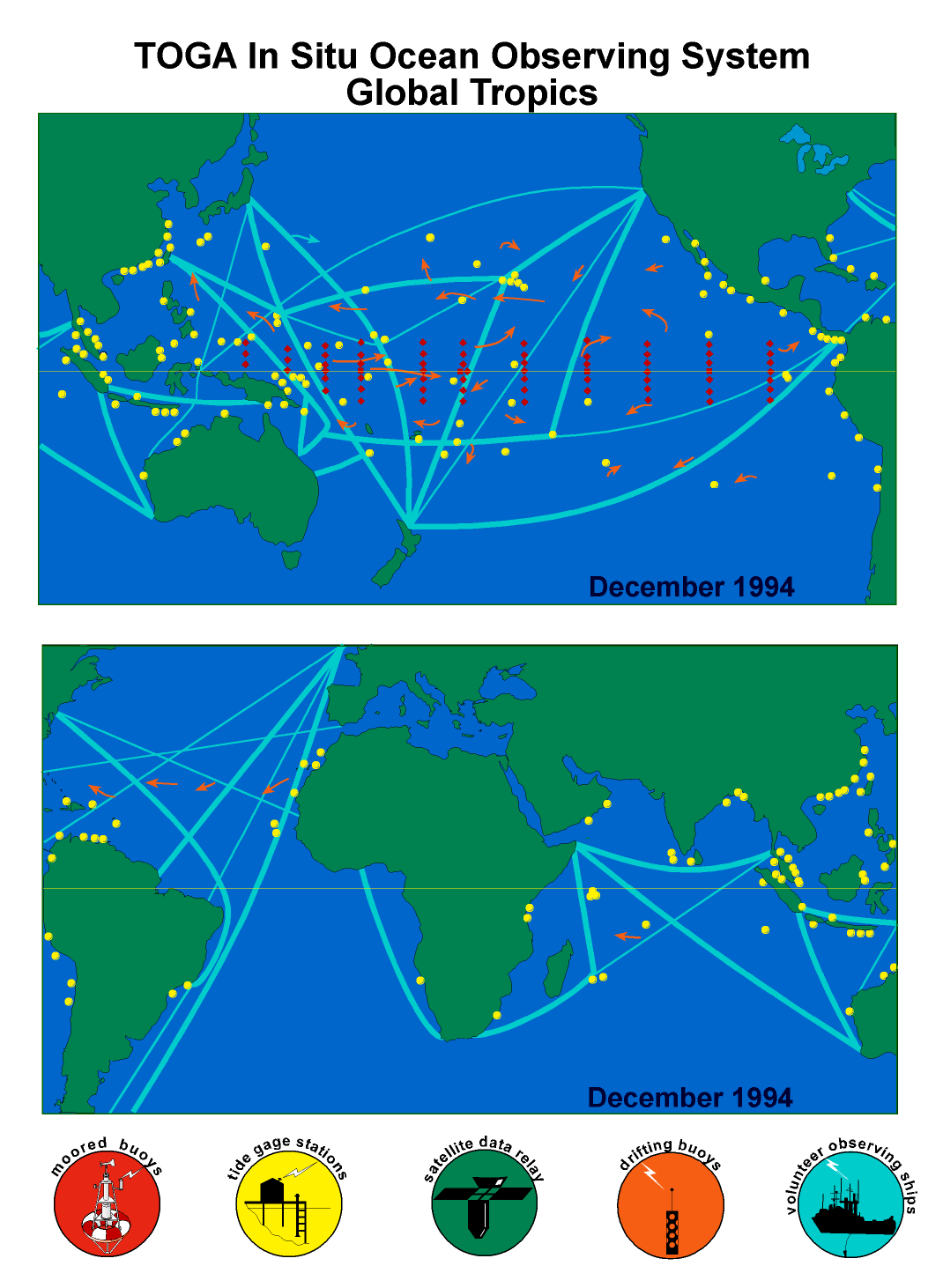
Figure 3: The in situ TOGA Ocean Observing System in its final configuration in December 1994. (top) Pacific Ocean, (bottom) Indian and Atlantic Oceans. Symbols are as in Figure 2.
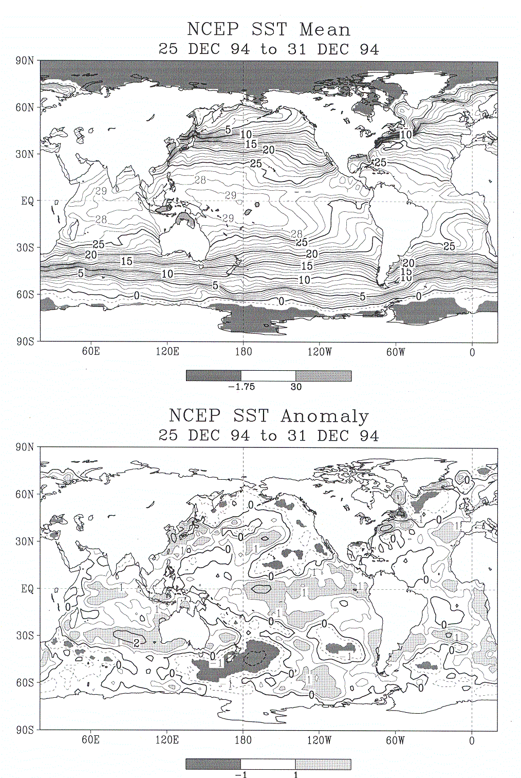
Figure 4: (top) SST weekly mean and (bottom) anomaly for December 25–31, 1994. The contour interval is 1°C, except there are two extra contours at ±0.5°C in Figure 4 (bottom). Negative contours are dashed. Heavy contour lines are used every 5°C in Figure 4 (top) and every 2°C in Figure 4 (bottom). In Figure 4 (top) the heavy shading at values < –1.75°C approximates the sea ice coverage. The anomalies are computed as departures from the monthly climatology of Reynolds and Smith [1995], which was interpolated to the weekly time period.
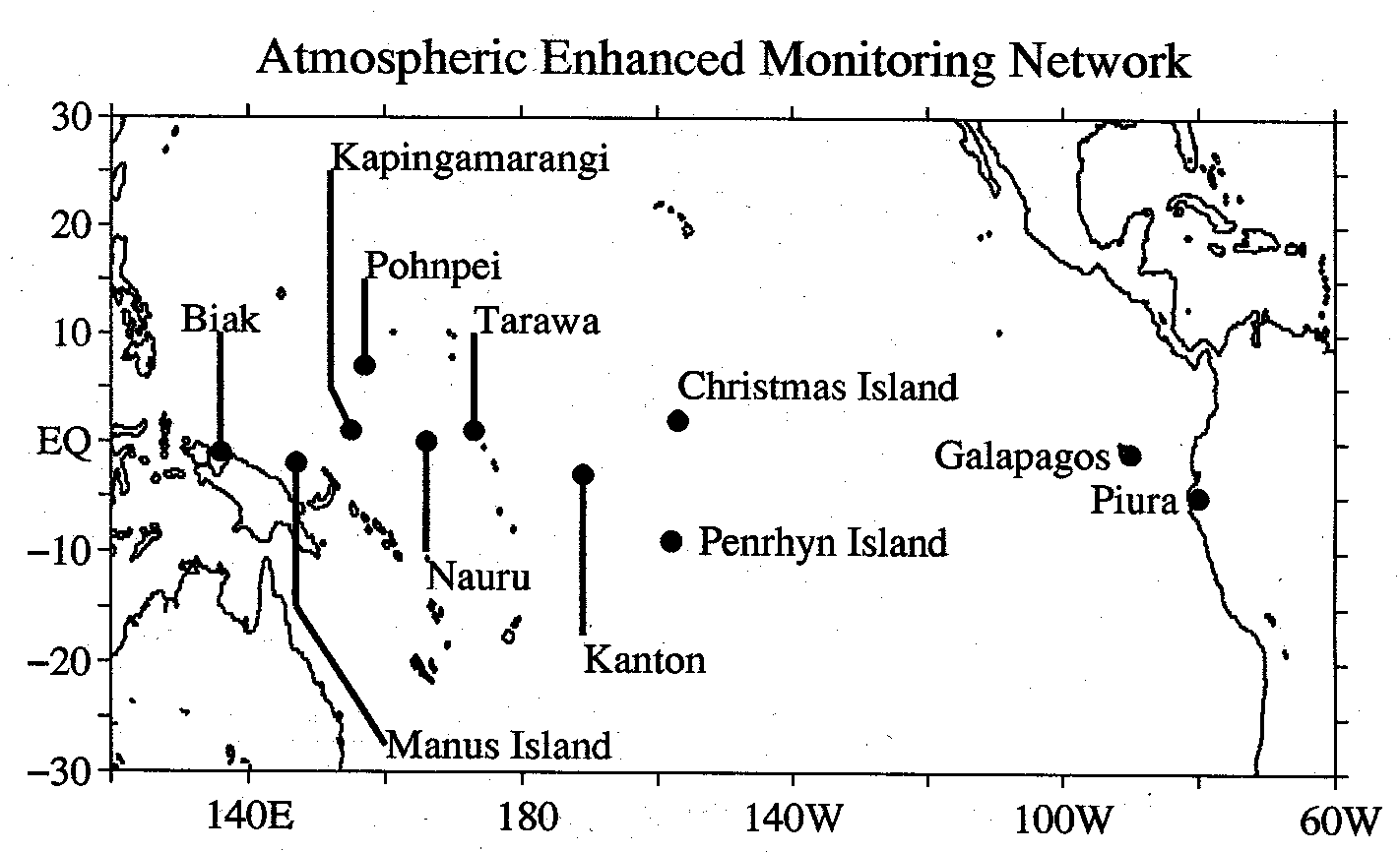
Figure 5: Map of the tropical Pacific Ocean basin
showing the locations of wind profilers and conventional upper air sounding
systems used for enhanced atmospheric observations during TOGA. Shown are VHF
and UHF profiler sites at Biak (Indonesia) and Christmas Island (Kiribati);
stand-alone VHF sites at Pohnpei (Federated States of Micronesia) and Piura
(Peru); stand-alone UHF profiler sites at Tarawa (Kiribati) and San Cristobal
(Galapagos Islands); and integrated sounding systems (ISS) at Manus Island (Papua
New Guinea), Kapingamarangi (Kiribati), and the island Republic of Nauru. The
ISS system consists of a UHF profiler integrated with a balloon sounding system
and surface meteorological instruments; the ISS sites at Manus Island, Nauru,
and Kapingamarangi were established as part of TOGA COARE. World Weather Watch
sites using conventional sounding systems were maintained at Tarawa, Kanton
(Kiribati), San Cristobal, and Penrhyn. Not shown is the World Weather Watch
(WWW) upper air sounding station site established by TOGA at Gan (0.5°16.1 S, 73°16.1E) in the Maldive Islands.
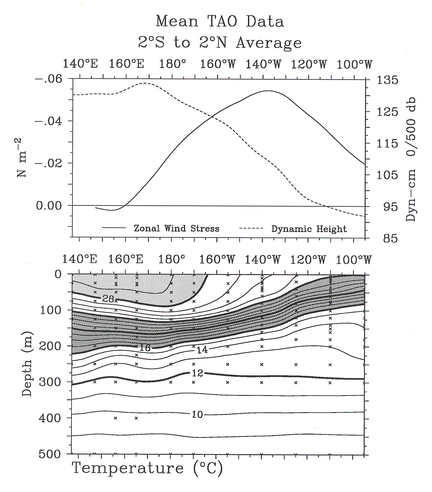
Figure 6: Zonal section of mean temperature averaged between 2°N and 2°S on the basis of available TAO time series data in 1980–1996. Also shown is the corresponding mean zonal wind stress (computed using a constant drag coefficient of 1.2 × 10⁻³) and dynamic height 0–500 dbar (computed using mean temperature/salinity relationships based on work by Levitus and Boyer [1994] and Levitus et al. [1994a]). Crosses indicate depths and longitudes where temperature data were available. An average at a particular location was computed only if a minimum of 2 years of data was available.
![]()
Figure 7: Mean temperature for the period 1985–1994 on four well-sampled XBT lines. Typically, 120 or more realizations of the quasi-synoptic temperature field were obtained during the decade for each section. The standard deviation of seasonal-to-interannual temperature variability during 1985–1994 from the Australian ocean thermal analysis system [Smith, 1995b] is indicated by shading. Westernmost section is at the top, easternmost at the bottom.
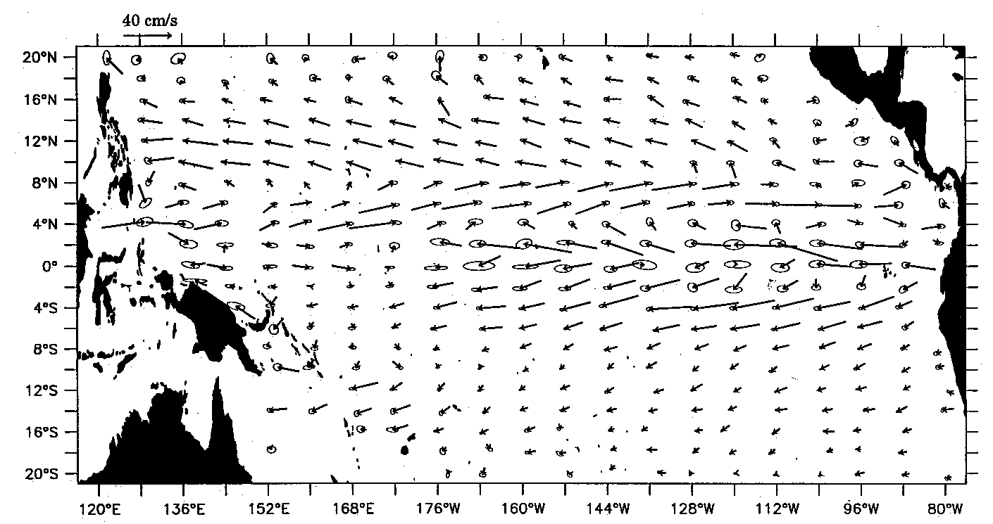
Figure 8: Mean surface layer (15 m) circulation in the tropical Pacific based on Surface Velocity Program drifter data for the period 1988–1994. The ellipse at the end of each vector is the 95% confidence interval.
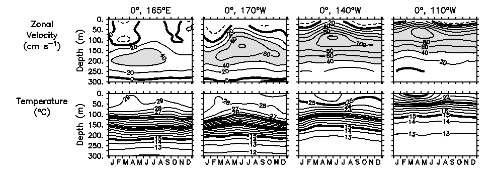
Figure 9: Mean seasonal cycles of temperature and zonal velocity at four sites along the equator based on multiyear analyses (1980–1994 at 110°W, 1983–1994 at 140°W, 1988–1994 at 170°W, and 1986–1993 at 165°E). The 110°W, 140°W, and 165°E analyses are updated versions of those found in work by McPhaden and McCarty [1992] and McCarty and McPhaden [1993]. The 170°W analysis is based on data presented by Weisberg and Hayes [1995], extended through 1994.
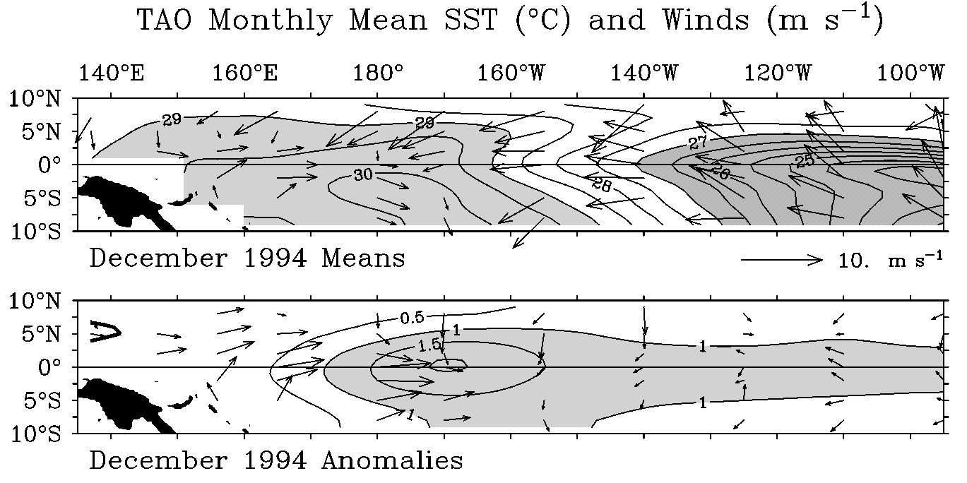
Figure 10: Wind vectors and SSTs from the TAO array for December 1994. (top) Monthly means; (bottom) monthly anomalies from the COADS wind climatology and NCEP SST climatology (1950–1979). SSTs warmer than 29°C and colder than 27°C are shaded; SST anomalies >1°C and <-1°C are shaded.
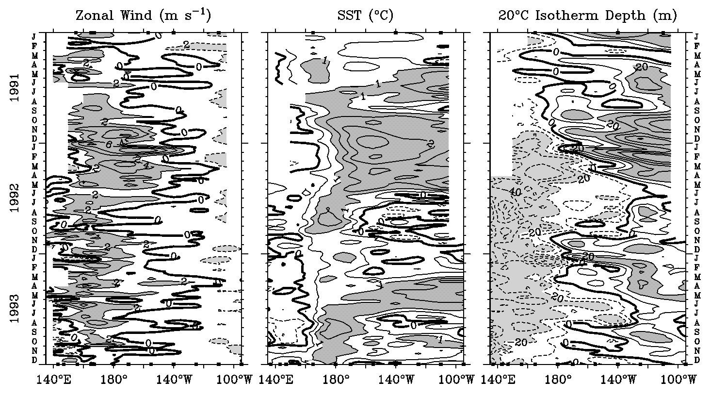
Figure 11: Time-longitude sections of anomalies in surface zonal winds (in m s-1), sea surface temperature (in °C), and 20°C isotherm depth (in meters) for January 1991 to December 1993. Analysis is based on 5-day averages between 2°N and 2°S of moored time series data from the TAO Array. Anomalies are relative to monthly climatologies cubic spline fitted to 5-day intervals (COADS winds, Reynolds and Smith [1995] SST, CTD/XBT 20°C depths). Shading indicates anomaly magnitudes > 2 m s-1, 1°C, and 20 m for winds, temperatures, and 20°C depths, respectively. Positive winds are westerly. Squares on the top abscissa indicate longitudes where data were available at the start of the time series, and squares on the bottom abscissa indicate where data were available at the end of the time series.
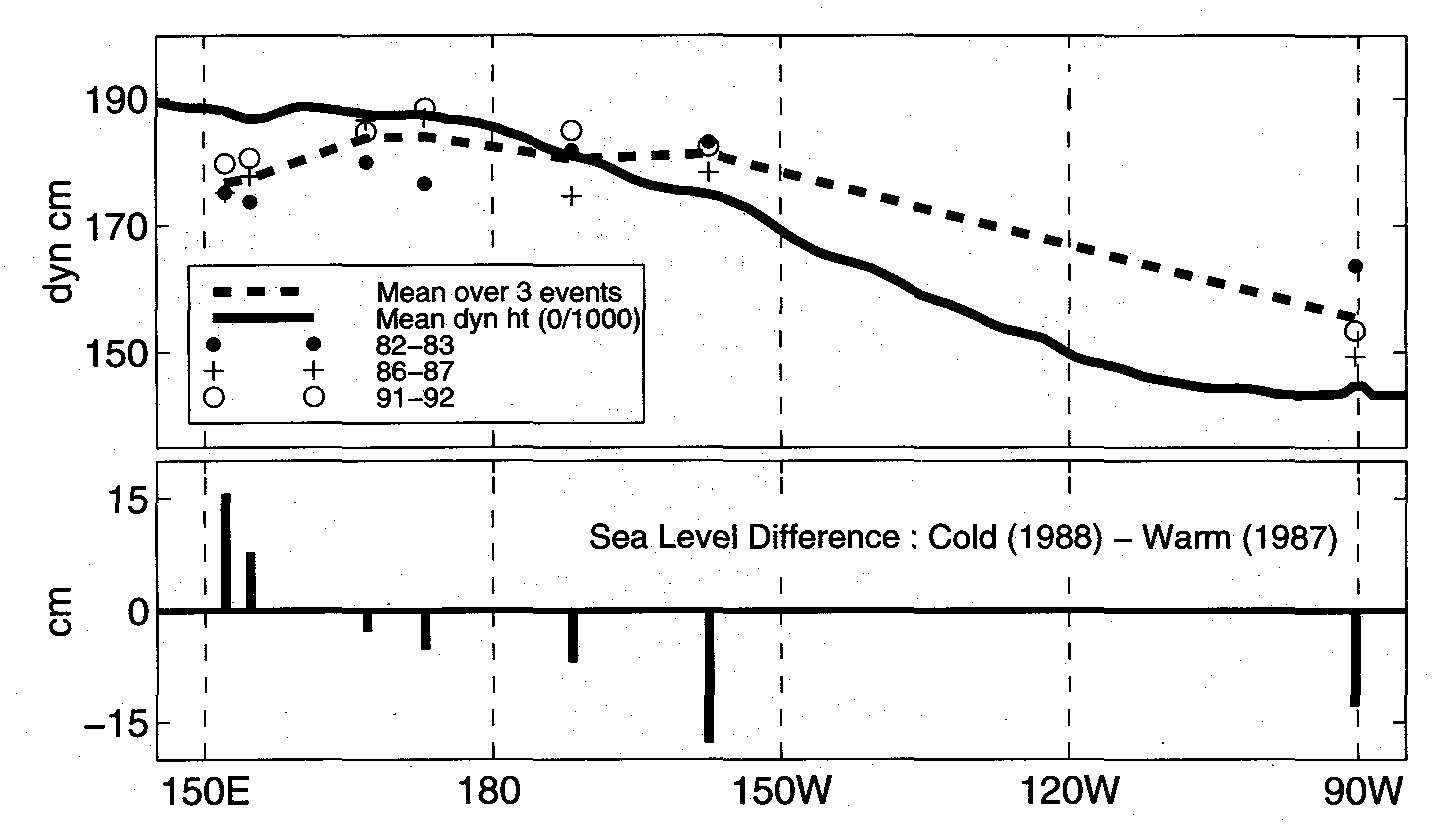
Figure 12: Zonal slope of sea surface height along the equator. Sea level anomalies from the 1975–1987 mean seasonal cycle were taken from seven locations near the equator: Rabaul (4°S, 152°E), Kapingamarangi (1°N, 155°E), Nauru (0.5°S, 167°E), Tarawa (1°N, 173°E), Kanton (3°S, 172°W), Christmas Island (2°N, 157°W), and the Galapagos Islands (0.5°S, 90°W). These anomalies were added to the mean dynamic topography difference (0–1000 dbar) computed from the Levitus and Boyer [1994] and Levitus et al. [1994a] temperature and salinity climatologies in order to calculate absolute heights. (top) Mean conditions during three warm events are shown as solid circles (June 1982 to May 1983), crosses (January to December 1987), and open circles (June 1991 to May 1992). The heavy solid line is the long-term mean conditions taken from the Levitus climatology. (bottom) Warm and cold conditions are contrasted by showing the difference (the vertical bars) of the mean sea level anomaly in 1988 (cold) minus the mean sea level anomaly in 1987 (warm).
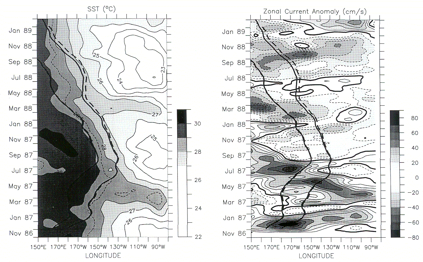
Figure 13: (left) Longitude-time distribution of 4°N–4°S averaged SST. Contour interval is 1°C, except for the 28.5°C isotherm. Superimposed as thick lines are the trajectories of two hypothetical drifters moved by 4°N–4°S averaged surface current anomalies derived from Geosat data (thick solid lines correspond to the total currents; thick dashed lines correspond to the Kelvin and Rossby wave contributions). (right) Longitude-time distribution of 4°N–4°S averaged surface current anomaly derived from Geosat. Contour interval is 10 cm s-1. Solid (dashed) lines denote eastward (westward) current anomalies. Thick solid and thick dashed lines are as in Figure 13 (left). From Picaut and Delcroix [1995].
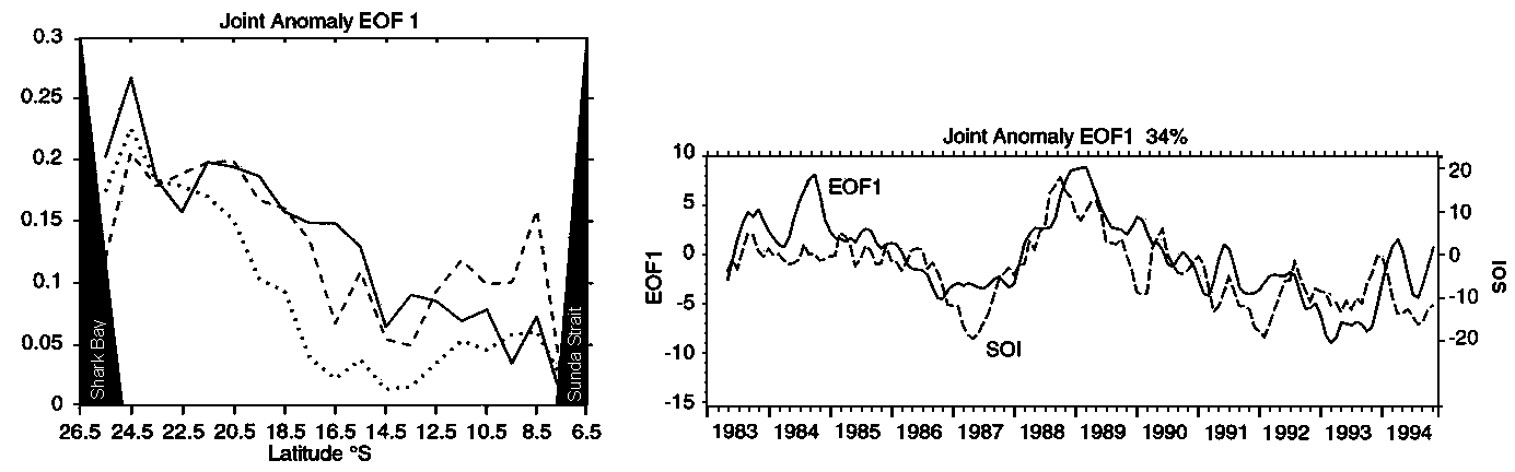
Figure 14: Joint empirical orthogonal functions (EOFs) of anomalies of SST, dynamic height (0–400 dbar) and depth of the 20° isotherm on a frequently repeated XBT line between Shark Bay (westernmost point of Australia) and Sunda Strait (western end of Java). (left) The first EOF (34% of the variance) shows the ENSO signal entering the Indian Ocean along the coast of Australia. (right) The temporal coefficients of the first EOF are highly correlated with the Southern Oscillation Index (SOI). From Meyers [1996].
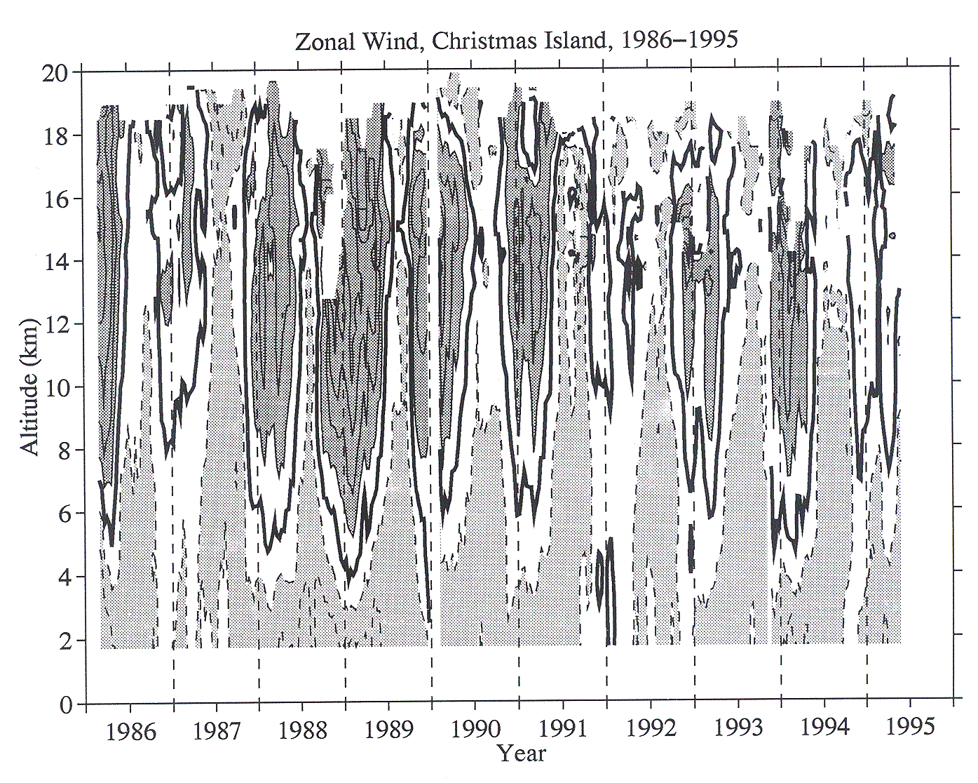
Figure 15: Time-height cross section of Christmas Island zonal winds, April 1986 to April 1995. After Gage et al. [1996b].
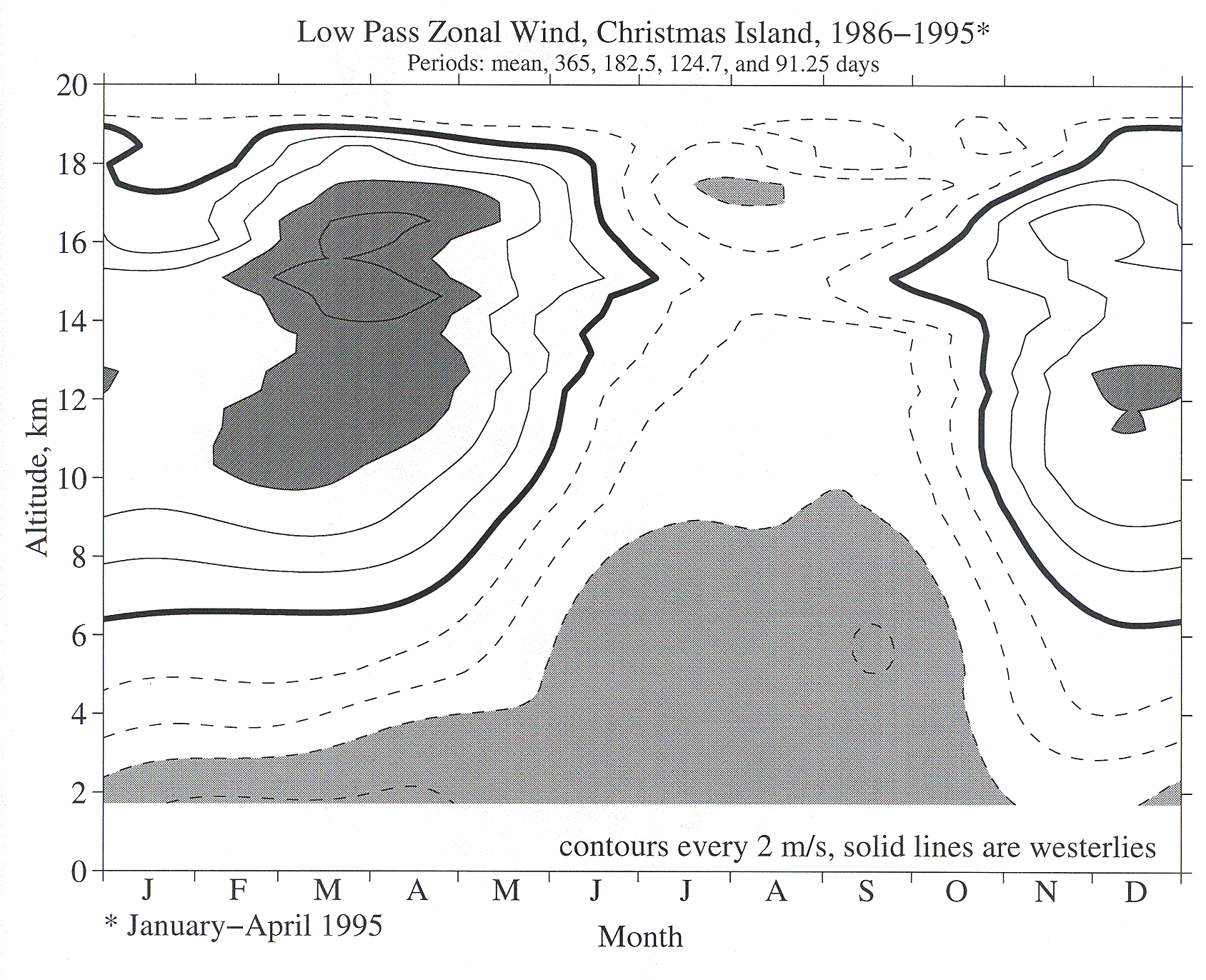
Figure 16: Low-pass-filtered composite annual cycle of zonal winds observed at Christmas Island. After Gage et al. [1996b].
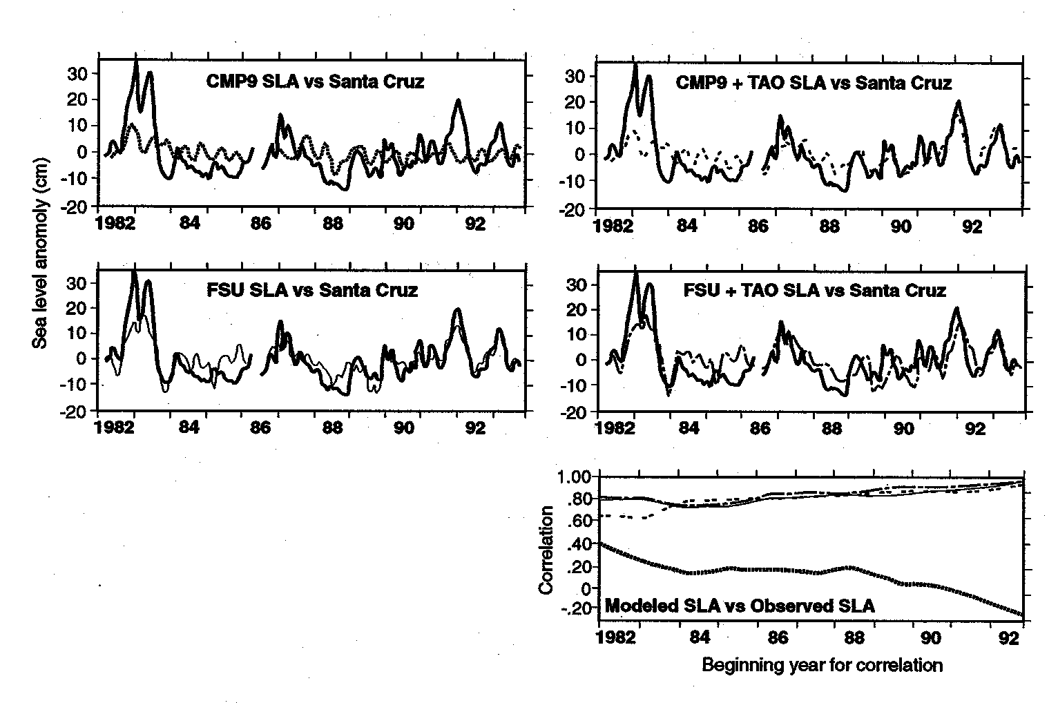
Figure 17: Modeled sea level anomaly (SLA) versus observation at Santa Cruz, Galapagos Islands. (top left) CMP9 (dotted line) simulation versus observations (solid line). (top right) Same as Figure 17 (top left), but for CMP9 plus TAO (dashed line). (middle left) Same as Figure 17 (top left), with FSU (thin line). (middle right) Same as Figure 17 (top left), with FSU plus TAO (dot-dash line). (bottom) The correlation coefficient between the modeled and observed sea level anomalies as the time over which the correlation is computed progressively reduced by 1 year from its starting date (labeled on abscissa) to 1993. For example, the point labeled 1987 represents the cross correlation from 1987 through 1993.
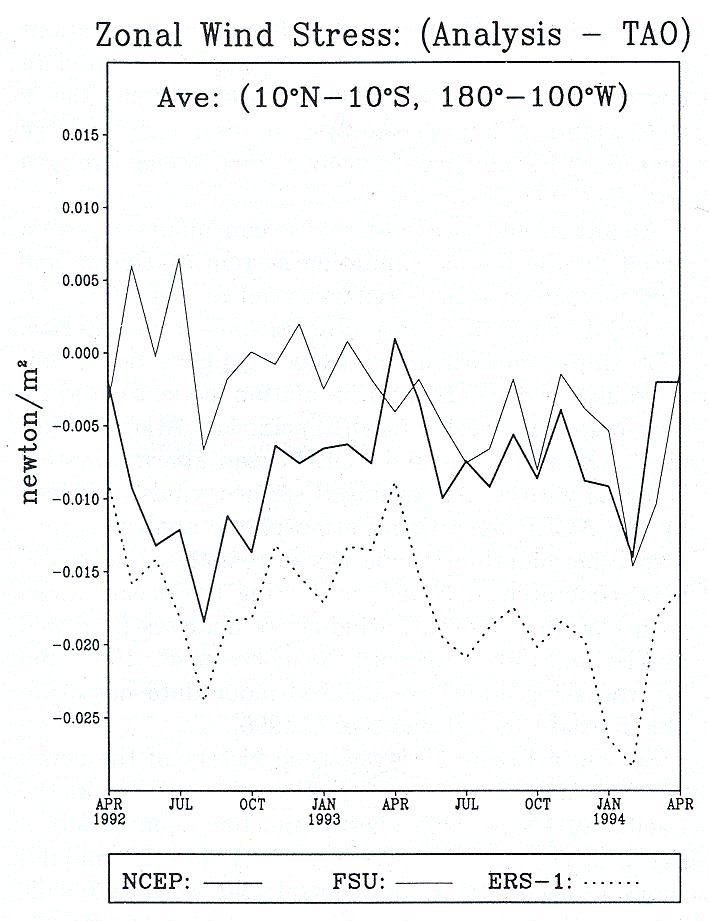
Figure 18: Zonal wind stress differences relative to TOGA-TAO for three products: NCEP, FSU, and ERS-1. The differences are averaged over 10°N to 10°S and 180° to 100°W. After Ji and Leetmaa [1997].
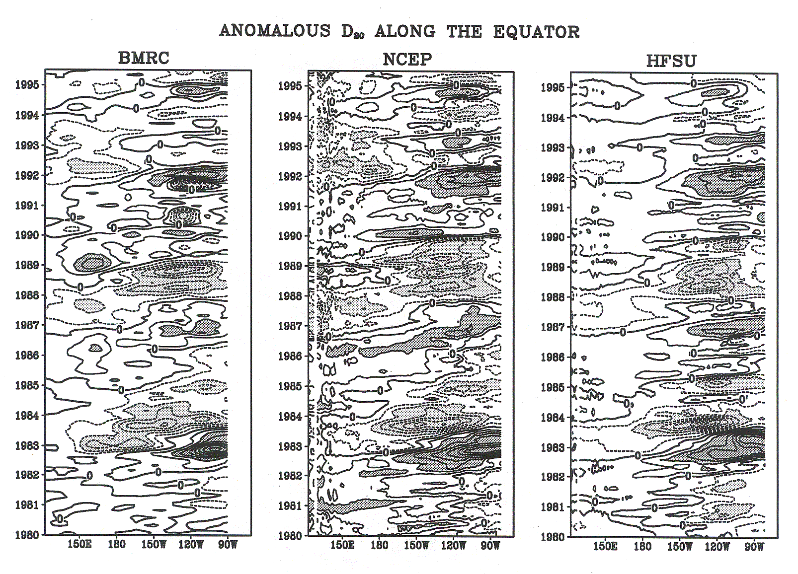
Figure 19: Anomalous depth of the 20° isotherm along the equator for the Pacific produced (left) by BMRC, (middle) by the NCEP ocean analysis system, and (right) by an ocean model simulation forced with monthly surface wind analyses from FSU. The contour interval is 10 m. Anomalies greater (less) than 20 m (-20 m) are indicated by dark (light) shading. From Ji and Leetmaa [1997].
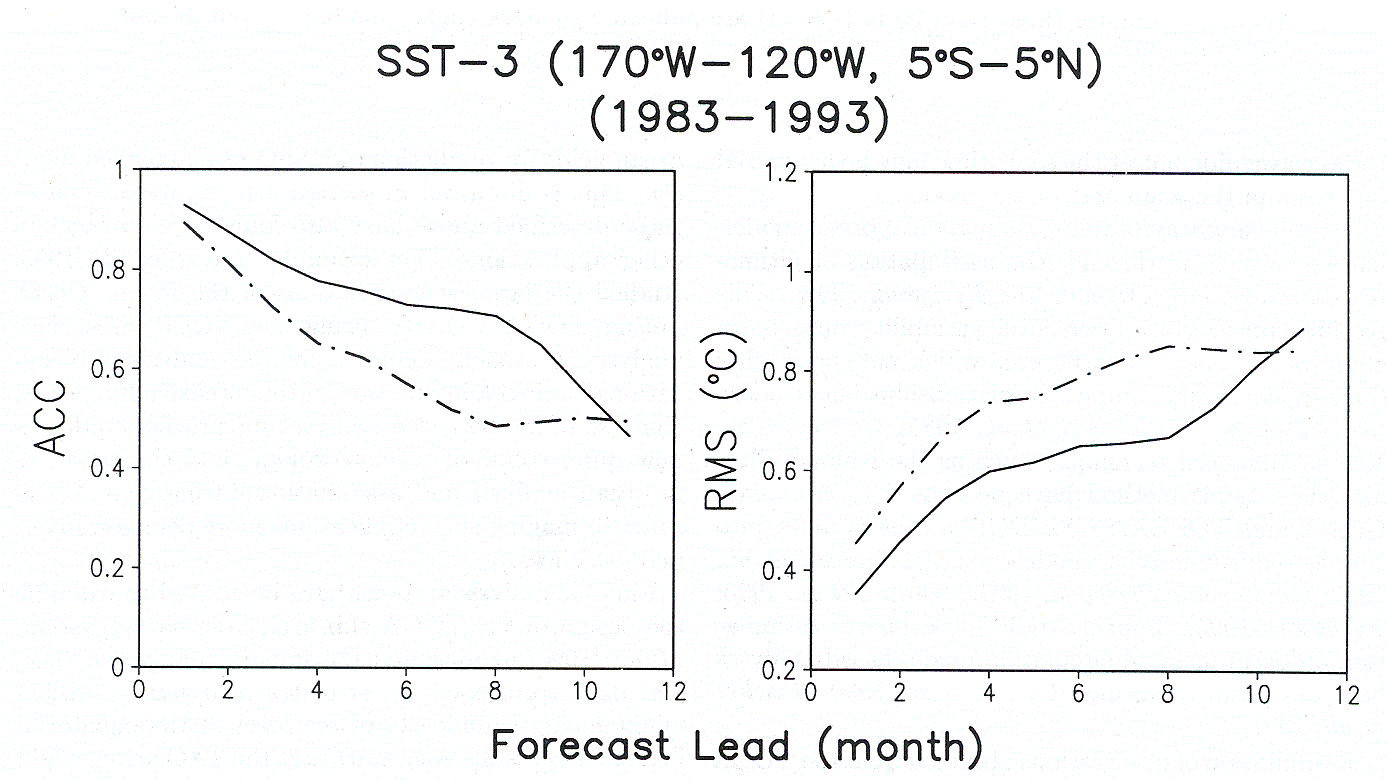
Figure 20: (left) Anomaly correlation coefficients and (right) rms errors between forecasts and observations for area-averaged SST anomalies in the eastern equatorial Pacific region between 170°–120°W and 5°S–5°N. Solid (dash-dot) lines are for forecasts initiated from ocean initial conditions produced with (without) subsurface data assimilation.
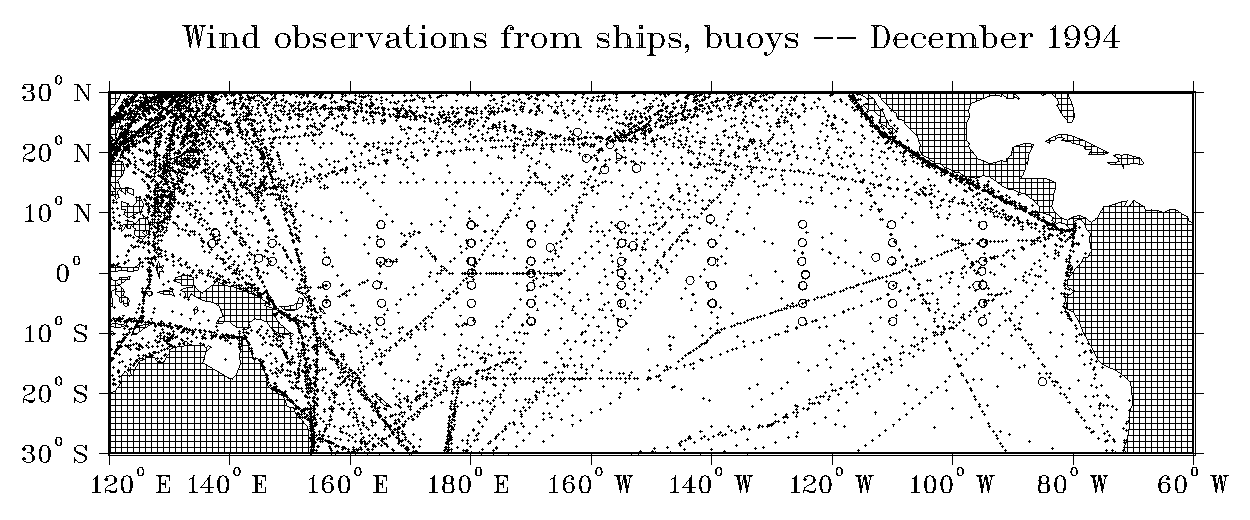
Figure B1: GTS ship (small solid dot) and buoy (open circles) wind reports used in the Florida State University Pacific surface wind analysis for the month of December 1994. In the latitude band 10°N–10°S a total of 6970 observations were reported; 3809 of these reports (55%) were from TAO buoys (data courtesy of D. Legler, 1997).
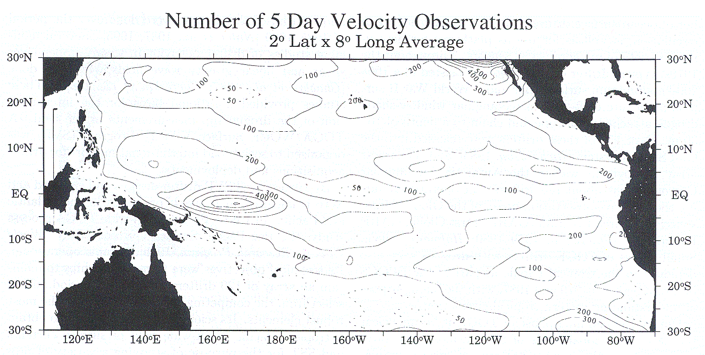
Figure B2: Number of 5-day observations of velocity observed in 2° latitude × 8° longitude areas from surface drifters between January 1, 1979, and December 31, 1995, in the tropical Pacific. The total number of 5-day observations is 81,589. The maximum number of 5-day observations possible in any given box is 1098.
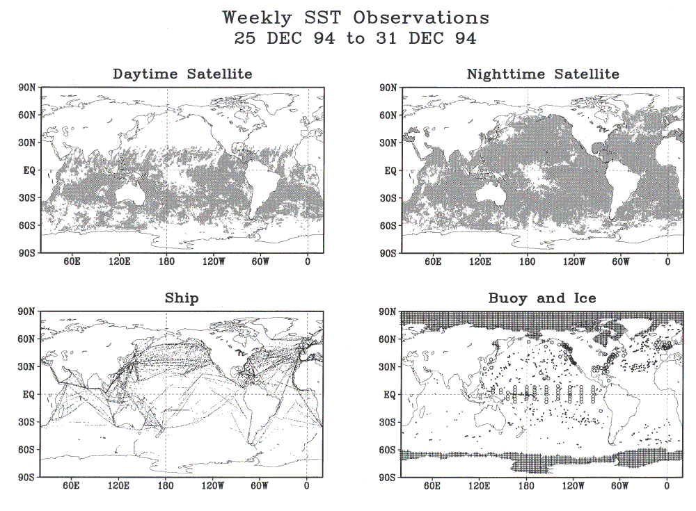
Figure C1: Number of SST observations for the week of December 25–31. (top) Regions on a 1° grid where the number of daytime or nighttime AVHRR retrievals is three or more. (bottom) The distribution of ship, buoy, and simulated ice SSTs. In Figure C1 (bottom right) the moored buoys are indicated by a circle, the drifting buoys by a dot, and the ice by a plus.
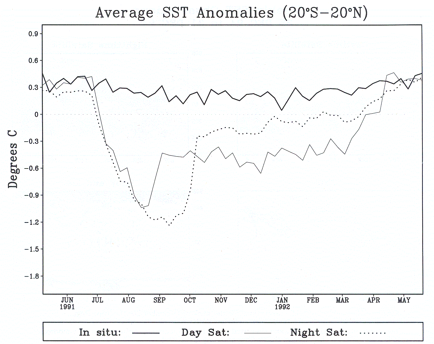
Figure C2: SST anomalies obtained from weekly in situ, daytime, and nighttime satellite observations. The anomalies are averaged between 20°S and 20°N from May 1981 to May 1992 [from Reynolds, 1993].
Figure C3: Sea level time series computed from Geosat, ERS-1, and TOPEX/POSEIDON altimeter data (solid line) near the Honiara tide gauge (dashed line) in the western tropical Pacific (taken from Lillibridge et al. [1994]).
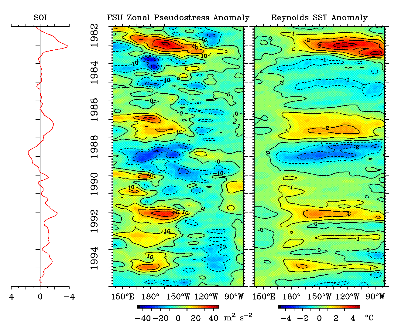
Plate 1: Time-longitude plots of zonal pseudostress (in m2 s-2) and SST (in °C) between 2°N and 2°S along the equator from 1982–1995. Pseudostress time series are from the Florida State University (FSU) analyses [Stricherz et al., 1992], and the SST is from Reynolds and Smith [1994]. Also shown is the Southern Oscillation Index (SOI) for the same time period. The SOI, defined as the normalized difference in surface pressure between Tahiti, French Polynesia and Darwin, Australia is a measure of the strength of the trade winds, which have a component of flow from regions of high to low pressure in the tropical marine boundary layer. High SOI (large pressure difference) is associated with stronger than normal trade winds and La Niña conditions, and low SOI (smaller pressure difference) is associated with weaker than normal trade winds and El Niño conditions. All time series have been smoothed with a 5-month triangle filter (roughly equivalent to a seasonal average). The FSU pseudostress and Reynolds SST have also been smoothed zonally over 10° longitude.
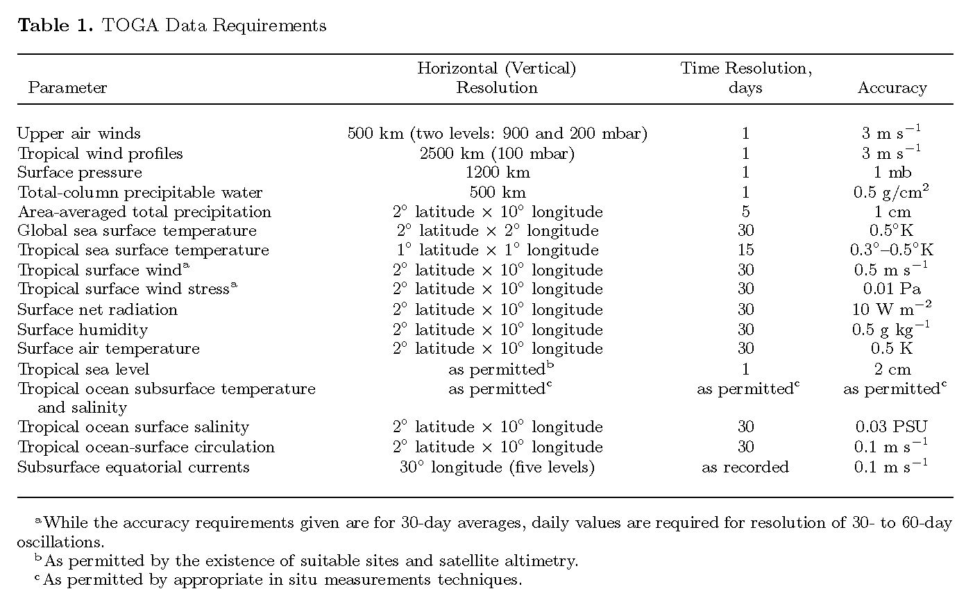
Table 1. TOGA Data Requirements
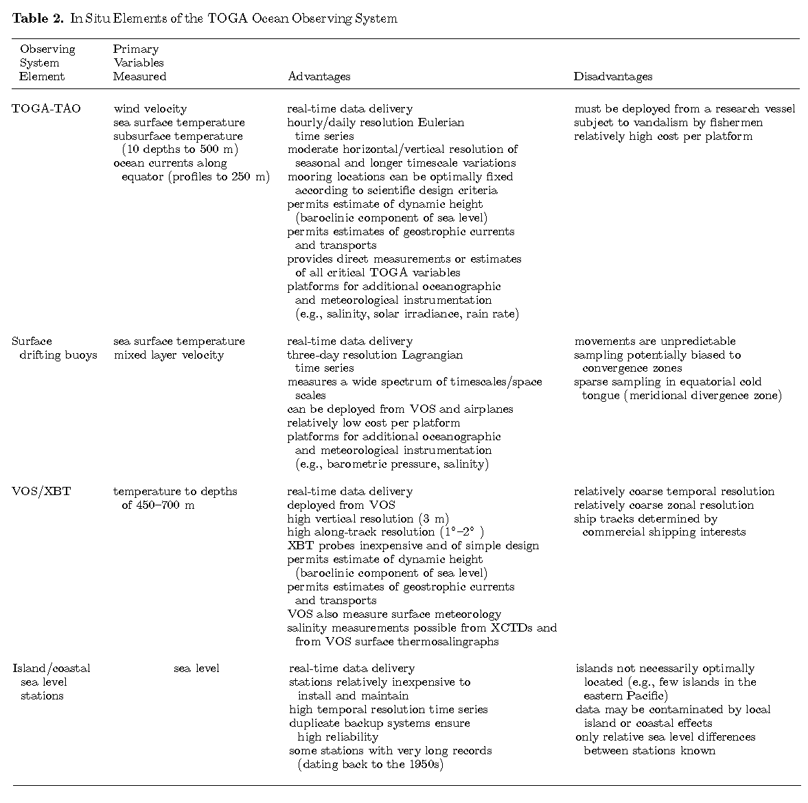
Table 2. In Situ Elements of the TOGA Ocean Observing System
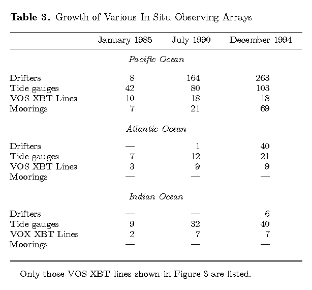
Table 3. Growth of Various In Situ Observing Arrays
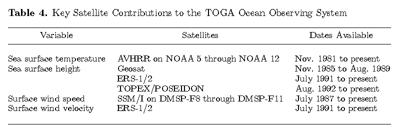
Table 4. Key Satellite Contributions to the TOGA Ocean Observing System
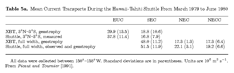
Table 5a. Mean Current Transports During the Hawaii-Tahiti Shuttle From March 1979 to June 1980
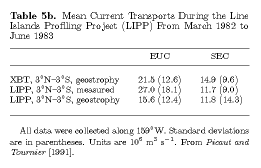
Table 5b. Mean Current Transports During the Line Islands Profiling Project (LIPP) From March 1982 to June 1983
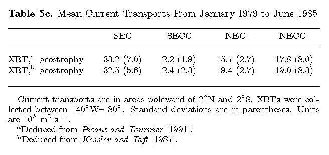
Table 5c. Mean Current Transports From January 1979 to June 1985
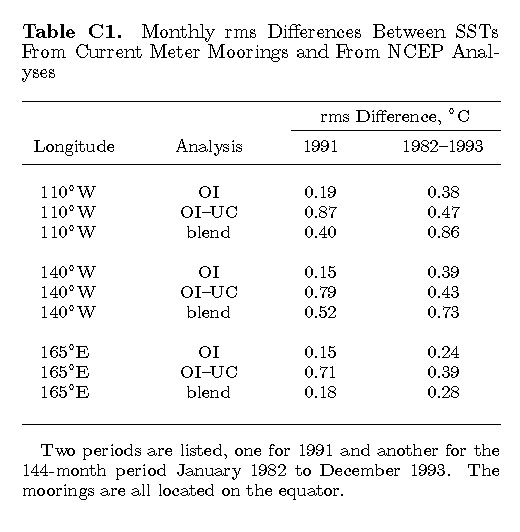
Table C1. Monthly rms Differences Between SSTs From Current Meter Moorings and From NCEP Analyses
Return to References or go back to Abstract