The circulation of the eastern tropical Pacific: A review

W. S. Kessler

NOAA/Pacific Marine Environmental Laboratory, Seattle, Washington

Prog. Oceanogr., 69, 181–217, 2006.
Copyright ©2006 Elsevier Science Ltd. Further electronic distribution is not allowed.

1. Introduction

Spurred by the valuable tuna fishery of the region, a major effort was undertaken in the late 1950s and early 1960s by the Scripps Institution of Oceanography, in collaboration with national and international fisheries research organizations, to observe the eastern tropical Pacific. Indeed, the opportunity presented by this program brought Klaus Wyrtki to Scripps in 1961 (Von Storch et al., 1999). The seminal papers describing the circulation, dynamics and water properties of the region came out of this project (Reid, 1948; Cromwell, 1958; Wooster and Cromwell, 1958; Cromwell and Bennett, 1959; Roden, 1961, 1962; Bennett, 1963; Wyrtki, 1964, 1965, 1966, 1967; Tsuchiya, 1975). Following this productive period, relatively few in situ physical observations have been made; for example more than 30% of the total modern database of hydrographic profiles in the region east of 130°W between 30°S and 30°N were taken before 1975. The literature shows a similar pattern. Until the recent interest in the eddies off Central America (see Willett et al., 2006), there was a significant fall-off in publications discussing the circulation of the region after the mid-1960s; except for an ongoing effort by researchers at CICESE (Baumgartner and Christensen, 1985; Badan-Dangon et al., 1989) and studies of equatorial dynamics based on the TAO (Tropical Atmosphere Ocean; see Hayes et al., 1991) moorings and cruises along 110°W (e.g., McPhaden and Hayes, 1990), only scattered papers were published on the low-frequency regional circulation between 1967 and 2002. Since the Wyrtki papers of the 1960s are still widely cited as the authoritative description of the regional circulation (e.g., Badan-Dangon, 1998), it seems useful to review what was known at that time and what has been learned since to confirm, supplement, update or contradict that description. The circulation reviewed here is related to the physical forcing and water mass characteristics described in reviews of the east Pacific atmosphere (Amador et al., 2006), the variability of the surface heat fluxes (Wang and Fiedler, 2006), the hydrography of the eastern Pacific (Fiedler and Talley, 2006), the regional signatures of interdecadal variations and climate change (Mestas-Nuñez and Miller, 2006), and the mesoscale eddies (Willett et al., 2006).

Much of the descriptive and dynamical study of the tropical Pacific from the 1970s to the 1990s focused on the long zonal scales of the central Pacific, where the winds, thermal structure and currents are nearly a function of latitude alone, and where a zonal-average meridional section is a useful approximation. By contrast, in the east the presence of the American continent is the dominant factor, producing strong meridional winds and zonal variations of forcing and properties. In addition, the necessity for the large zonal transports to be redistributed as the currents feel the coast produces a complicated three-dimensional structure. The focus of this review is on the circulation in the region where the shape of the continent and the continentally influenced winds are the dominant factor; for recent discussions of circulation in the central Pacific see McPhaden et al. (1998); Lagerloef et al. (1999); Johnson and McPhaden (1999); Johnson et al. (2002). The region affected by the continent extends as far as 2500 km west of the coast of Central America, though much less than this north of 20°N or south of the equator. A physically based way to define the region is where the southeast corner of the mean North Pacific Gyre does not reach into the large bight between central Mexico and Ecuador; this definition has the boundary stretching south from the tip of Baja California approximately along 110°W. This conforms to the eastern edge of the gyre-like winds of the North Pacific and of the zonally oriented Intertropical Convergence Zone (ITCZ) that is typical of the central Pacific (Fig. 1; see Section 4.1). The wind forcing associated with the ITCZ between the two subtropical highs produces the long ridges and troughs that bound the zonal currents of the central Pacific (South Equatorial Current (SEC), North Equatorial Countercurrent (NECC), and North Equatorial Current (NEC)). East of 110°W this ridge-trough system breaks down (Fig. 2, and see Fiedler and Talley, 2006), allowing meridional flows and strong zonal gradients of both winds and currents, with southerly cross-equatorial winds and a complex system of currents that exchange mass meridionally. The region between the tip of Baja California and the equatorial cold tongue also roughly coincides with the east Pacific warm pool (Wang and Fiedler, 2006), so it makes sense to discuss it as a distinct dynamical and climatic regime. To the south, equatorial dynamics tie the entire equatorial region firmly together, so the eastern equatorial Pacific's circulation cannot be considered in isolation. As Wyrtki (1966) noted, physical features like the cold tongue extend far out into the central Pacific and do not have a welldefined boundary on their west. In addition, Kelvin waves efficiently carry the signatures of west-central Pacific wind anomalies to the east, and determine a large fraction of east Pacific thermocline depth variations (e.g., Spillane et al., 1987; Kessler and McPhaden, 1995b). However, winds in the far eastern equatorial Pacific are distinct in being characterized by a strong southerly cross-equatorial component (Fig. 1), unlike the nearly zonal winds of the central basin, which suggests a qualitatively different dynamical regime in the east. In keeping with the definition used for the region north of the equator, we will define the eastern part of the equatorial Pacific as the longitude range where the meridional component of the wind is larger than the zonal component; this boundary is approximately at 110–105°W (Fig. 1). Much field study over the past two decades has been done in connection with the TAO mooring at 110°W, so this choice allows incorporation of that work in the review.

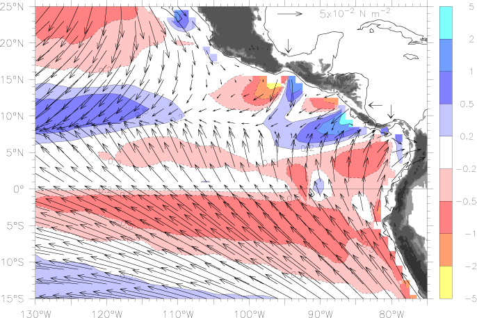
Fig. 1. Mean wind stress (vectors) and wind stress curl (colors) averaged over August 1999–July 2002. Blue shading shows positive curl (upwelling in the northern hemisphere) and red negative curl, in units of 10 Nm, with (stretched) color key at right. The scale vector is in the Gulf of Mexico. Gray shading on land indicates altitudes greater than 250 m. The three mountain gaps referred to in the text are marked with arrows on the Atlantic side; from north to south these jets are denoted Tehuantepec, Papagayo, and Panama.

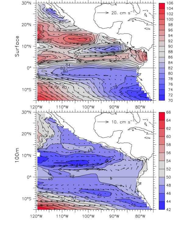
Fig. 2. Mean dynamic height and geostrophic currents relative to 400 m. Top: surface. Bottom: 100 m. Red colors indicate high dynamic heights, blue low (color scales on right). The contour interval is 2 dyn cm. The scale vector for each plot is located in the Gulf of Mexico. Geostrophic current vectors are omitted within ±3° latitude.

2. What Wyrtki knew: The picture in the mid-1960s

During the mid-1960s, Wyrtki assembled the physical picture that had been gained under the Scripps cruises and longterm ship-drift records into three partly overlapping papers (Wyrtki, 1965, 1966, 1967). These summary papers represented his own work, and also that of Cromwell (1958), Wooster and Cromwell (1958), Knauss (1960), Roden (1962), Bennett (1963) and other Scripps collaborators. The historical shipdrift data (Cromwell and Bennett, 1959) tracked the surface currents and their seasonal variations in fair detail, and a series of expeditions conducted by Scripps, by government fisheries vessels, and under the CalCOFI program (see Table 1 of Wyrtki, 1966) provided a few hundred bottle casts and a few thousand bathythermograph profiles in the region.

This by-modern-standards-limited dataset enabled Wyrtki to draw the schematic seasonal surface circulation shown in Fig. 3, which is in broadscale agreement with results from the picture that would be drawn from the much more comprehensive modern surface drifter data set (Fig. 4). Among the important features recognized were the winter extension of the California Current southward past Cabo San Lucas, the strengthening of the North Equatorial Countercurrent (NECC) during August–January, and its drastic weakening in the east during boreal spring (Section 4.2), the mean Costa Rica Dome and associated Costa Rica Coastal Current (CRCC) (Section 4.1), and the cyclonic circulation in the Panama Bight (Fig. 4). Roden (1962) had shown the relevance of wind-driven Sverdrup dynamics to the eastern Pacific, especially in realizing that the Peru Undercurrent must be rather strong (making the total transport southward along the Peru coast), though he was limited by the poor quality of wind datasets available. Important missing elements in the mid-1960s picture were the weakness of the South Equatorial Current (SEC) in a narrow band right at the equator (especially during March–July) (Section 4.3) and the connection between the NECC and the SEC (which is still poorly known). Although Peru upwelling was well known and equatorial upwelling was surmised (Cromwell, 1953), the three-dimensional structure of the eastern Pacific was not well understood. Wyrtki was aware of the sharp SST front bordering the north edge of the equatorial cold tongue (Cromwell, 1953), but the tropical instability waves (TIW) that distort the front on monthly timescales (Baturin and Niiler, 1997; Chelton et al., 2000) were not discovered until the advent of satellite SST in the late 1970s (Legeckis, 1977). Similarly, the strong eddies that occur under the winter winds blowing through the gaps in the Central American cordillera (Willett et al., 2006) were not described until the 1980s, although the effects of these winds on the shape of the local thermocline were described by Roden (1961). The Costa Rica Dome was an early focus because of the importance of the tuna catch there, and Wyrtki (1964) devoted an entire paper to it. However, the lack of appreciation at that time for the role of wind-driven vorticity dynamics led him to drastically underestimate the upwelling into the Dome and to misunderstand its mechanism (see Section 4.1).

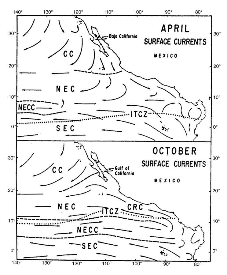
Fig. 3. Annual cycle surface circulation based on ship-drift records (after Baumgartner and Christensen, 1985, which was adapted from Wyrtki, 1965). Current abbreviations are: California Current (CC), North Equatorial Current (NEC), North Equatorial Countercurrent (NECC), South Equatorial Current (SEC) and Costa Rica Coastal Current (CRC). The Intertropical Convergence Zone (ITCZ) is marked by a dotted line. Dashed lines around the NECC show its varying extent.

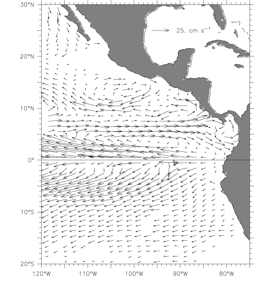
Fig. 4. Mean surface circulation from surface drifters. Vectors were left blank if either the total count of samples in that 1° × 1° box was less than 10, or if fewer than 4 months of the year were represented. The scale vector is located in the Gulf of Mexico.

A key factor that enabled a description of the circulation was the then-recent discovery of the equatorial undercurrent (EUC; Cromwell et al., 1954; also see McPhaden, 1986 and Montgomery, 1959 for historical overviews). By the time Wyrtki wrote his summary papers in the early 1960s, several expeditions had confirmed and added detail to Cromwell's discovery (Knauss, 1960), and it was obvious that the large eastward transport of the EUC must play a major role in the mass balance of the eastern Pacific. Previously, it had been hard to account for the westward growth of the SEC, which is much larger than the Humboldt Current that apparently fed it. Knauss (1960) estimated the EUC transport at 39 Sv, and Wyrtki (1966) drew a schematic circulation (reproduced here as Fig. 5a), in which about 20 Sv of EUC water went into the SEC near the Galapagos. However, though realizing that substantial EUC water must feed the SEC, Wyrtki (1966) thought that a large upwelling transport was impossible, commenting "the amount of water upwelled along the equator certainly does not exceed a few 10 cm/s [Sv], otherwise the thermal structure would break down". Therefore, he postulated that the EUC water must move into the lower levels of the SEC without rising to the surface. Wyrtki corrected himself 15 years later with a since-confirmed estimate of 50 Sv of upwelling over 170–100°W, based on the meridional divergence of Ekman and geostrophic transports (Wyrtki, 1981). A remaining item of confusion that was not cleared up until much later concerned the spreading of isotherms about the EUC (Fig. 6 and Section 4). It was thought at the time that this spreading must be a signature of vertical mixing, which seemed reasonable in such a strong current. However, turbulence measurements beginning with Gregg (1976) showed that mixing is in fact very weak at the EUC core; instead being strong in the stratified region above the current where it serves to maintain the balance between large upwelling transport and downward heat flux (see Gregg, 1998 for a review of the turbulence observations, and Fiedler and Talley, 2006 for a description of the EUC hydrography).

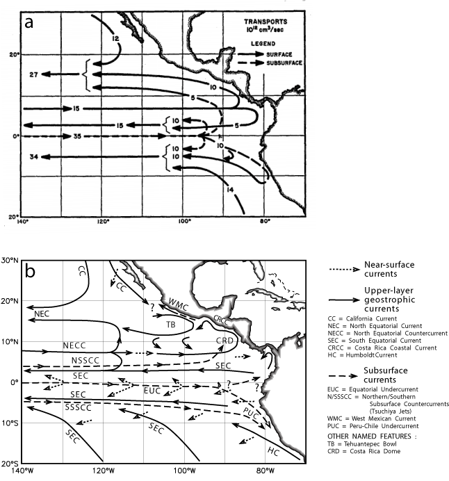
Fig. 5. Schematic three-dimensional circulation in the eastern tropical Pacific. (a) After Wyrtki (1966). (b) The circulation based on modern data. The legend at the right lists the names of currents and features referred to in the text. Several question marks indicate regions where the interconnections among the currents remain unknown (see text).

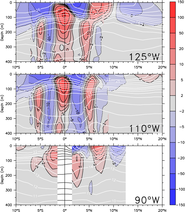
Fig. 6. Mean meridional sections of temperature (white contours) and zonal current (color shading, where red is eastward and blue westward; cm s) at the three longitudes listed in the lower right corner of each panel. At 125°W and 110°W, directly measured currents are shown within ±8° latitude (see Appendix C.1); elsewhere the currents are geostrophic.

3. Data and methods

Although much of this paper reviews published work, additional calculations are reported based on ocean and wind observations. These data sets and their processing are described in detail in the Appendix. The principal thermal data set used to construct the average annual cycle of thermocline depth and the resulting geostrophic currents (Section 4.2) is a compilation of historical XBT profiles by Donoso et al. (1994), and referred to here as the "AOML XBT data" (Appendix A.1). In some regions, directly measured velocities are available from the ships servicing the TAO moorings and from a few of the moorings themselves (Appendix C.1). The ship velocities are referred to here as the "Johnson ADCP data" (Johnson et al., 2002), and the moored velocities as the "TAO data". Surface drifters (Appendix C.4) also produce useful direct velocity measurements, however in many cases the very-near-surface currents sampled by the drifters are quite different than the much thicker currents due to thermocline topography, and do not represent the major transport patterns, especially under strong winds (e.g., the difference between Figs. 2 and 4, south of the equator). We also note that very few drifters have been deployed near the coast of central Mexico, so these data do not provide a good picture of the crucial region where the California Current meets the tropics. Satellite scatterometer winds are used to estimate Ekman pumping and to force a Rossby wave model (Section 4.2.1). These winds were sampled by the European Research Satellite (ERS) over the period 1991–2001, used to construct an average annual cycle, and also by the Quikscat (Seawinds) instrument for the period August 1999 through July 2002 (Appendix B). These are referred to here as the "ERS" or the "QuikSCAT" winds, respectively. Supplementary data sets (satellite SST, and sea surface height (SSH) from satellite altimetry) are used to augment the principal data sources for particular purposes (Appendix C).

In several plots, the geostrophic circulation is shown as contours of dynamic height, which is a convenient quantity because its contours are streamlines of the geostrophic flow, and its cross-stream gradient measures the flow speed; these relations are seen as the current vectors parallel to the dynamic height contours in Fig. 2. Dynamic height measures the vertically integrated density anomaly, expressing the fact that a less dense (i.e., warmer or fresher) water column of a given total mass stands taller than a denser one. Because deep flows are observed to be small in most regions, it is reasonable to assume that there are no pressure gradients at some deep reference level, otherwise these gradients would drive currents. Since pressure measures the mass of water above that level, equal pressure implies that the mass of water columns above the reference level must be the same, and thus the density of each column determines its height. Dynamic height is scaled to accurately represent sea surface height relative to a reference level. In the tropics, the density contrast between adjacent columns arises primarily because of thermocline variations: a water column with deep thermocline has a thick upper warm layer and is overall warmer than a column with shallow thermocline; thus it has higher dynamic height.

4. Observations

4.1. Mean circulation

The mean density structure and consequent geostrophic circulation are shown in plan view and as meridional sections in Figs. 2 and 6, respectively, and as a schematic in Fig. 5b (see also Fiedler and Talley, 2006).

4.1.1. Transition between the eastern and central Pacific

At the western edge of the region (125°W; Fig. 6, top), the well-known zonal currents of the central Pacific are seen. In the south, the thermocline slopes down into the bowl of the South Pacific subtropical gyre; south of about 10°S, sampling is insufficient to do more than sketch the broad westward and equatorward flow of the SEC that extends to about 25°S (Fig. 5b). The SEC is broken up into many branches and filaments whose structure and timescales remain poorly observed and understood (Morris et al., 1996; Kessler and Gourdeau, 2006). Near the equator, the two main lobes of the SEC at about 3°S and 3°N have mean surface speeds near 50 cm s; it is not known why they extend so deeply into the water column. The sharp SST front occurs along the axis of the northern branch; because the front is advected ±200 km north and south on 20–30-day timescales by tropical instability waves (Baturin and Niiler, 1997; Willett et al., 2006), it appears heavily smoothed in a time average like Fig. 6. Surface flow at the equator is slightly westward in the mean (but reverses in boreal spring, see Section 4.3) above the eastward EUC, centered near 80 m depth at 125°W. The thermocline is quite tight from 14 to 24 °C at ±5° latitude, but spreads at the equator, implying eastward geostrophic flow (the EUC) with its maximum in the center of the spreading, and westward shear (the SEC) above.

The trough at 5°N and ridge at 10°N bound the eastward NECC, and the downward slope north of the ridge gives the westward NEC, which is the southern limb of the North Pacific subtropical gyre. Below the thermocline, the paired eastward currents at about 125–400 m depth near ±4–5° latitude, associated with the deep bowl of isotherms from 10 to 12 °C (Fiedler and Talley, 2006), are the Subsurface Countercurrents (SSCCs or Tsuchiya Jets) that originate in the far western Pacific (Tsuchiya, 1975; Rowe et al., 2000; McCreary et al., 2002).

Ekman surface currents diverge from the equator in both hemispheres above about 30 m depth, balanced by equatorial upwelling (Johnson, 2001). Fig. 4 shows that the surface flow direction is dominated by Ekman transport; almost 90° to the left of the main SEC flow, especially under the strongest trade winds just south of the equator (Fig. 1). The general downward tilt of the thermocline towards the west (Fiedler and Talley, 2006) results in equatorward geostrophic flow (Fig. 2, top) that supplies the upwelling.

All these currents can be seen entering and leaving the region at the western edge of Fig. 2, and this pattern continues westward across the entire basin. Fig. 6 (top) is similar to sections that would be made as far west as about 170°E, except that all the surface currents would be somewhat stronger and the entire structure deepening to the west (Wyrtki and Kilonsky, 1984; Taft and Kessler, 1991; Johnson et al., 2002; Fiedler and Talley, 2006).

4.1.2. The eastern tropical Pacific

East of 120°W the picture is much more complicated and includes substantial meridional flow that feeds and drains the outgoing and incoming zonal currents. The southeastern corner of the North Pacific subtropical gyre occurs where the California Current flows south along the coast of Baja California and gradually turns west to feed the NEC, though its path is partly indirect, depth-dependent, and seasonally varying. Below the thermocline (Fig. 2, bottom) the turn to the west is clear, but at the surface (top panel), geostrophic currents continue southeastward along the coast of Mexico. However, the Ekman transport in this region is westward (i.e., to the right of the wind vectors in Fig. 1) so the very-near-surface flow is southsouthwest (Fig. 4), approximately parallel to the deeper geostrophic contours (Fig. 2). Part of the shallow geostrophic California Current probably continues southeast around the thermocline bowl centered at 13°N, 105°W (discussed below), to feed the NEC by a second pathway at about 13°N (Fig. 2, top), predominantly in boreal spring (Fig. 7). The NEC is also fed by water that has flowed east in the NECC, which extends all the way to the coast in boreal fall, but greatly weakens near 110°W in spring (Fig. 7), as discussed further below. These seasonal changes were already recognized by Wyrtki in 1965 (Fig. 3), but Figs. 2 and 5b show that the source region of the NEC comprises a complex mingling of currents that have not yet been fully deciphered.

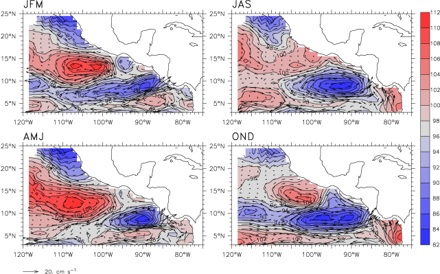
Fig. 7. Annual cycle of surface dynamic height and geostrophic current (relative to 450 m), shown as four average seasons. Red colors indicate high dynamic heights, blue low. The contour interval is 2 dyn cm. The scale vector for geostrophic currents is at lower left. The dynamic height contours shown here have very nearly the same patterns as contours of 20 °C depth for the corresponding season.

At 110°W, the structure of the EUC and SEC is similar to that at 125°W, though perhaps 20 m shallower, but the mean geostrophic NECC is nearly absent (Fig. 2, top and Fig. 6, middle). The ridge near 9–10°N that supports the NECC has almost completely flattened out (compare the isotherms in Fig. 6, middle vs. top). The weak eastward geostrophic flow found at 5–6°N is due to isotherm slopes below 13 °C; that is, associated with the Tsuchiya Jet and not the thermocline. Surface dynamic height has only a very small meridional pressure gradient between 5°N and 9°N at 110°W (about 2 dyn cm at 110 °W compared to about 14 dyn cm at 120°W; Fig. 2, top), as both the 10° ridge and 5°N trough nearly disappear. Much of the NECC splits, to turn south into the SEC and north into the NEC (note the dynamic height contours from 86 to 90 dyn cm turning north, and those from 94 to 98 dyn cm turning south between 120°W and 110°W, with only a small fraction of the geostrophic NECC continuing to the east). Similar patterns are shown in other climatologies (Strub and James, 2002b). This is a remarkable termination for a current well out in the interior basin. The mean drifter velocities, by contrast, show an apparently continuous NECC all the way from 120°W to the Costa Rica Dome (Fig. 4). The discrepancy is not due to sampling or other problems with the XBT data, as the directly measured currents show, if anything, a weaker mean surface NECC at 110°W (compare Fig. 6, middle, which uses directly measured currents south of 9°N, with Fig. 2, which is entirely geostrophic). Kessler (2002) noted that the Ekman flow under the region's southerly winds (Fig. 1) is strongly eastward, in part due to the small value of the Coriolis parameter this close to the equator. With reasonable assumptions about the Ekman depth (Ralph and Niiler, 1999), the Ekman currents account for nearly all the difference between the geostrophic (Fig. 2) and drifter (Fig. 4) depictions of the NECC at 110°W (see section 4b of Kessler, 2002). Thus the apparently continuous NECC seen by the drifters across 110°W is a near-surface Ekman feature that does not represent the geostrophic NECC that can be followed across the entire basin, and the NECC is therefore shown in Fig. 5b only as a near-surface current at 110°W. Since the Ekman flow is quite shallow the transport of the eastward jet in Fig. 4 is small, about 1 Sv over the width of the eastward current, compared to about 9 Sv for the geostrophic NECC at 125°W in Fig. 6. This mid-basin termination of the NECC is strongly seasonally modulated. In boreal spring, there is no eastward flow at all along 110°W anywhere south of the California Current (Fig. 7, lower left), whereas in boreal autumn and winter the NECC appears to flow all the way to the coast (right panels). The drifter seasonal cycle at 110°W shows the same pattern of variability, as do currents inferred from satellite altimetry (Strub and James, 2002b).

A striking bowl and dome are found in the mean dynamic height, centered at 13°N, 105°W and 9°N, 90°W, respectively (Fig. 2, top). (In the following, we will refer to these features as they appear in thermocline topography, not dynamic height; that is, the Costa Rica Dome at 9°N where the 20 °C isotherm rises to about 25 m, and the "Tehuantepec Bowl" at 14°N where 20 °C is at about 90 m. Note that the top panel of Fig. 2 is nearly equivalent to a map of the depth of the 20 °C isotherm which marks the thermocline, taking high dynamic height as corresponding to deeper isotherm depths.) Since the upwelling associated with the Costa Rica Dome produces a nutrient-rich environment that might support tuna and other fisheries, such as jumbo squid (Ichii et al., 2002), it has been studied much more intensely than the Tehuantepec Bowl, which does not even have a recognized name. These features appear to be the eastern ends of the thermocline trough and ridge that define the limits of the NEC across the basin, with the trough connecting to the center of the subtropical gyre and the ridge running along 9–10°N between the NEC and NECC all the way to the Philippines (Wyrtki, 1975b; Kessler, 1990). Notably, however, both the trough and ridge flatten near 110°W (as has been commented on above with respect to the NECC) before restrengthening near the coast and terminating in the nearly detached bowl and dome. They are clearly seen as counter-rotating eddies in the drifter (Fig. 4) and geostrophic (Fig. 2, top) velocity vectors. Although the Costa Rica Dome has a clear subsurface expression, extending much further to the west below the thermocline, the Tehuantepec Bowl is a shallow feature that is barely visible in the 100 m dynamic height (Fig. 2, bottom, and note that the 100 m dynamic height contours have a very similar pattern as the topography of the 12 °C isotherm).

Wyrtki (1964) noted the cool SST, low oxygen and high salinity and phosphate values in the center of the Costa Rica Dome as an indication of the upwelling of subthermocline water. Based on sections from several cruises, he estimated the current speed around the dome at about 20–50 cm s, which is comparable to modern estimates (e.g., Fig. 4). Wyrtki hypothesized that the centrifugal acceleration around the Costa Rica Dome would contribute an outward divergence and consequent upwelling. The upwelling estimated this way was quite small, less than 0.1 Sv, about 1/30th the modern value, although the values of all the terms Wyrtki used were similar to those that would be used today. Wyrtki's assumption that the reason for the upwelling was rapid rotation around the eddy as the NECC turned at the coast, was the source of the error. If he had scaled the terms he would have found that the centrifugal term is at least 10 times smaller than the geostrophic term. In fact, Costa Rica Dome upwelling is driven by the wind, as discussed in Section 4.1.3 below, which Wyrtki (1964) dismissed as weak and variable in the absence of sufficient observations, and he omitted wind forcing from his balance.

Northwestward flow on the east side of the Costa Rica Dome is known as the Costa Rica Coastal Current, with a mean speed of about 20 cm s, and a transport of more than 5 Sv (Fig. 2). In the mean, the CRCC continues along the coast into the Gulf of Tehuantepec, where its surface expression turns south to flow around the south side of the Tehuantepec Bowl. This northward extension is seasonally modulated as the Costa Rica Dome expands and contracts (Fig. 7). The CRCC extends quite deeply into the water column, with an appreciable flow below the thermocline (Fig. 2, bottom; and see also Fig. 8, bottom).

Fig. 8. Zonal sections of temperature (top) and meridional geostrophic current (bottom) along 8.5°N, from the coast (right edge) to 110°W. The contour interval for temperature is 1 °C from 8 to 14 °C, then 2 °C from 16 to 26 °C, then 1 °C from 27 to 29 °C; the 20 °C contour is darkened. In the bottom panel, northward current is indicated by solid contours, southward by dashed contours; the contour interval is every 5 cm within ±15 cm s, with additional contours at ±1 and 2, ±0.5 and ±0.2 cm s.

The paucity of ocean data along the southwest coast of Mexico has led to considerable confusion about the possible extension of the CRCC to the north. Wyrtki (1965) showed it continuing all the way up past the tip of Baja California in October (Fig. 3, bottom), and this interpretation has continued to be cited (Baumgartner and Christensen, 1985; Badan-Dangon, 1998). In the absence of velocity data, the fact that Gulf of California surface and subsurface water properties apparently originated in the central Pacific argued for the CRCC as the likely pathway (Badan-Dangon, 1998; Lavín et al., 2003). Nevertheless, neither the drifter (Fig. 4) nor geostrophic (Fig. 2) velocities indicate the mean surface CRCC continuing north past the Gulf of Tehuantepec. Instead, anticyclonic flow around the Tehuantepec Bowl produces a strongly southeastward current along the coast of Oaxaca into the Gulf of Tehuantepec that cuts off the CRCC and forces it to turn offshore (most of which eventually feeds the NEC). However, as noted above, the Tehuantepec Bowl is a shallow feature that occurs almost entirely above the 12 °C isotherm (near 200 m depth), and a thin finger of subthermocline poleward flow continues along the coast past the Gulf of Tehuantepec, as suggested by the 48 dyn cm contour extending along the coast as far as 100 °W (Fig. 2, bottom). Northwest of the Tehuantepec Bowl, a weak subthermocline dome and cyclonic circulation centered at 19°N, 109°W (Fig. 2, bottom) feeds California Current water to the coastal current. North of 17°N, the poleward coastal flow strengthens and extends to the surface to flow past Cabo Corrientes at 20°N with a mean speed of about 3 cm s and transport of 1–2 Sv. Numerical models indicate a similar pattern, but with larger current speeds (E. Beier, personal communication, 2004). Since this coastal current appears not to be simply a continuation of the CRCC, either in its velocity structure or in the water masses that it carries, we propose that it be called the "West Mexican Current" (WMC), which is shown schematically in Fig. 5b as an initially subsurface, then surface flow. With the sparse sampling in the region, the interconnections among the WMC, Tehuantepec Bowl and California Current remain poorly known, and we have indicated this uncertainty with a question mark in Fig. 5b.

The Tehuantepec Bowl weakens and retreats offshore during boreal summer (Fig. 7) (the dynamics that control this evolution are discussed below in Section 4.2.1). This weakens the coastal currents that block the surface CRCC, allowing additional leakage to the north around a weak feature along the Oaxaca coast in summer (Fig. 7). The 19°N, 109°W dome also becomes more evident at this time. During June–October, WMC speeds increase to more than 5 cm s, and it presumably transports more tropical water to the Gulf of California at that time (similar boreal summer poleward anomalies are also seen in currents diagnosed from satellite altimetric sea level (Strub and James, 2002b)). In Section 4.4 below, increased poleward transport to the Gulf of California during El Niño events is inferred; it is possible that these episodic surges could, over time, deliver a significant contribution to the water of tropical origin observed in the Gulf (Baumgartner and Christensen, 1985; Lavín et al., 2003). The single existing (published) hydrographic section across the WMC was made in December 1969, a few months after its usual seasonal maximum but at the height of an El Niño event (Roden, 1972). This showed a strong (46 cm s maximum), narrow (less than 100 km wide) surface-intensified current immediately against the coast at Cabo Corrientes, with northward flow to 700 m depth. Such a spatial pattern is consistent with the transient passage of an El Niño-generated coastal wave, though it is impossible to verify this.

4.1.3. Wind-driven dynamics of the mean circulation

The distinctive regional wind forcing is key to understanding the complex thermal structure of the region and the modification of the central Pacific zonal currents of the central Pacific near the continent. West of about 110 °W the characteristic central Pacific winds are seen (Fig. 1), with trade winds converging into a well-developed ITCZ. East of 110°W and north of the equator the pattern is quite different: instead of a zonally oriented ITCZ, the winds (and especially the wind curl) are dominated by jets blowing through three gaps in the Central American cordillera: Chivela Pass at the Isthmus of Tehuantepec in Mexico, the Lake District lowlands of Nicaragua inland of the Gulf of Papagayo, and the central isthmus of Panama where the Panama Canal was built (Fig. 1).

The wind stress curl is Curl() = /x - /y, where the components of the wind stress vector are and ; the curl expresses the rotation a vertical column of air would experience in a wind field that varies in space. The Central American wind jets extend at least 500 km into the Pacific and produce distinctive curl dipoles as wind strength decreases away from the jet axis: each jet has a region of positive curl on its left flank and negative curl on its right. (In the mean, the wind jets are more clearly defined by their associated curl dipoles than in the vector winds themselves; Fig. 1.) The magnitudes of these curls are at least as large as that of the ITCZ. Positive curl on the south flank of the Papagayo jet is enhanced and extended to the west because of the westerly winds south of the jet (Mitchell et al., 1989). The three wind jets are known to vary on short (weekly) timescales, especially in association with winter high pressure systems transiting North America (Chelton et al., 2000a,b), producing oceanic eddies of various types (Willett et al., 2006). For present purposes, we are interested in the jets' impact on the low-frequency dynamics, in which Ekman pumping due to their curl is the main factor.

Ekman pumping occurs because the winds and therefore the Ekman transport vary spatially, which produces convergences and divergences in the upper layer. As a consequence, the thermocline must rise or fall to conserve mass, so Ekman pumping is interpreted as a vertical velocity at the base of the surface layer. Zonal and meridional Ekman transports are (U = /f ,V = -/f ), where f is the Coriolis parameter and the density. The divergence of the Ekman transports (U/x + V/y) equals the wind stress curl divided by f , (where f is for the moment taken as constant). The Ekman pumping velocity Curl()/f , is of fundamental importance for the ocean circulation because it produces thermocline depth variations and resulting pressure gradients, which consequently produce geostrophic flow. For example, under northern hemisphere wind jets like those west of Central America, the Ekman transport is to the right of the wind direction, and is largest at the jet axis. Approaching the jet from its left, the Ekman transport is increasing, so on this side of the jet it is divergent, leading to upwelling. To the right of the jet axis, the Ekman transport is decreasing, and is thus convergent (downwelling). The curl dipoles seen in Fig. 1 thereby produce the thermocline bowls and domes, and the corresponding highs and lows in dynamic height (Fig. 2, top).

The consequences of Ekman pumping go beyond changing the thermocline depth, however. On a rotating planet, a locally still water column has the rotation rate ("vorticity") about its vertical axis equal to the local value of the Coriolis parameter divided by two (thus it is zero at the equator and grows in magnitude towards the poles). If the column is lengthened or shortened by Ekman pumping at the top, its vorticity will be changed in proportion to its cross-sectional area. Stretching produces increasing vorticity because the column becomes narrower and the same angular momentum is achieved by a faster rotation. In the absence of other forces or friction, a stretched column would experience a rotational acceleration. Thus the wind stress curl can be seen as imposing its rotation directly on the ocean, through the intermediary mechanism of Ekman pumping, which illustrates the connection between rotation and stretching (and is why Ekman divergence is proportional to the wind stress curl). In steady state (where total vorticity is conserved) a local increase in vorticity can be balanced by moving poleward, where the vertical component of the earth's rotation (the planetary vorticity) is larger. This is the basis of the Sverdrup relation, V = Curl(), where = df/dy is the meridional gradient of the Coriolis parameter and V is the total meridional (Sverdrup) transport (Sverdrup, 1947). It expresses the fact that meridional motion is equivalent to a change in rotation rate. For example, under positive curl, as occurs on the south flank of the Papagayo jet, Ekman pumping lifts the thermocline and thus stretches the water column beneath. The vorticity of the column increases, and in steady state it must move north to a latitude where its spin equals the planetary vorticity.

The region of positive wind curl on the south flank of the Papagayo jet (Fig. 1) produces especially strong upwelling (10–20 m month, comparable to equatorial upwelling) because the Ekman transport is northward under the easterly jet itself at 10–11°N and southward under the westerly winds at 6–8°N. As a result of this surface divergence, the thermocline is lifted and the water column beneath is stretched, forming the Costa Rica Dome at 9°N (Fig. 8, top, shows a zonal slice and Fig. 6, bottom, a meridional slice through the center of the dome). The thermocline dome produces a cyclonic eddy-like geostrophic circulation at the surface (Figs. 4 and 2 (top)), but no dome is seen below the shallow thermocline. Instead, subthermocline isotherms slope up to the west over a broad region to at least 105°W (Fig. 8, top; and see Fiedler and Talley, 2006), thus the resulting geostrophic flow deeper than about 50 m under the dome is all northward (Fig. 8, bottom, or Fig. 2, bottom). This thick subthermocline flow dominates the vertical integral, and total transport is northward across the whole dome region to at least 99°W, quantitatively consistent with the Sverdrup relation under positive curl (Kessler, 2002). The cyclonic eddy circulation of the dome is found to be a very shallow feature. Thus both the rotating dome and the northward flow beneath it are part of the ocean response to the Papagayo jet.

Knowing the vertical structure of geostrophic transport (from XBT data) allows the structure of vertical motion below the directly wind-driven Ekman layer to be inferred (if both v and w are assumed to be zero at 450 m); this is found to be a transport of about 3.5 Sv upward across the 17 °C isotherm into the dome, where it diverges in the Ekman outflow (Kessler, 2002). The dome is one of the few places in the ocean where upwelling arises mostly from below the thermocline (equatorial upwelling draws water primarily from the upper levels of the thermocline), and thus constitutes a perhaps-important means of communication from the intermediate to the surface layer. Wyrtki (1964) did not realize the importance of these vorticity dynamics because the existence of the Papagayo wind jet and its curl were not known at the time, and because the very sparse thermal observations available concentrated on the position of the surface dome itself and did not extend west of about 91°W, so the clue of northward transport under the dome remained unknown.

It has not been possible to construct a heat balance for the dome because the surface flux terms are so poorly known, and vary strongly on short timescales (Chelton et al., 2000b). However, it is clear that the upwelling transport diagnosed in the Costa Rica Dome implies a large downward mixing of heat to maintain a steady balance, otherwise the isotherms would continue to be advected upward. High wind speeds under the Papagayo jet provide a plausible source of this mixing, but a quantitative assessment remains to be accomplished.

Costa Rica Dome upwelling and subsurface northward transport are linked with the northern Tsuchiya Jet that flows across the entire Pacific at about 4°N, 150–200 m depth (Fig. 6). The northward flow under and to the west of the dome seen in Fig. 8 is in fact the Tsuchiya Jet turning abruptly away from the equator (Fig. 2, bottom, and note the disappearance of both Tsuchiya Jets at 90°W, compared to the sections further west in Fig. 6). About half the roughly 7 Sv transport of the northern Tsuchiya Jet upwells into the Costa Rica Dome, while the other half turns and flows west into the lower reaches of the NEC (Fig. 2, bottom; note the large Tsuchiya Jet approaching the dome and weaker flow leaving the region at these depths, Kessler, 2002). The mechanism driving the Tsuchiya Jets remains in question, but recent theory suggests that the northern branch is in fact a consequence of Costa Rica Dome upwelling (McCreary et al., 2002), as an example of a "-plume" (Stommel, 1982). The southern branch may be similarly driven by upward motion across a broader region of the southeast Pacific (the negative curl along 5°S in Fig. 1, plus Peru upwelling), with a subthermocline dome reported near 10°S, 85°W (Voituriez, 1981); this is probably the long feature stretching from 105°W to the coast along 5–12°S in Fig. 2, bottom. The Atlantic also has Tsuchiya Jets flowing into upwelling in the Guinea and Angola Domes (Mazeika, 1967). Thus Costa Rica Dome upwelling appears to be the northeast Pacific instance of a more general phenomenon.

The mean ocean response to the Tehuantepec and Panama wind jets is also consistent with the Sverdrup relation: northward geostrophic transport is found under their left flanks and southward under their right (Kessler, 2002). Unlike Papagayo, for these jets the downwelling curl is larger than the upwelling curl (Fig. 1). In the Gulf of Tehuantepec, the mean curl dipole produces the northward bulge of the Costa Rica Dome (note the 88–92 dyn cm contours in Fig. 2, top, that go north under the upwelling curl to the east of Tehuantepec and south to its west). The Tehuantepec Bowl is consistent with a linear response to the downwelling curl stretching west from the right flank of the Tehuantepec wind jet (Kessler, 2002).

Interpreting the mean and low-frequency evolution of the Tehuantepec Bowl from sparse XBT data is tricky because it is in an area where anti-cyclonic eddies pass each winter (Giese et al., 1994; Willett et al., 2006), and it could be that the apparent mean bowl was simply a reflection of sampling many such eddies. In addition, the strength of the short timescale eddies suggests that nonlinear terms would be important. However nonlinearity seems not to be dominant for the mean circulation, which can be reasonably well diagnosed based on linear Sverdrup dynamics (Kessler, 2002). In the Panama Bight, the curl dipole produces a cyclonic circulation with northward flow along the Colombian coast, and (rather weak) southward flow at 85–90°W (Fig. 2). One of the first modern dynamical formulations for the vertical velocity due to the curl was developed by Stevenson (1970) to interpret the circulation in the Panama Bight. He estimated upwelling velocities of few m day in the central gulf, and showed a rough consistency of upwelling due to the wind curl with the cyclonic geostrophic gyre. Cool SST along the coast of Colombia might be a response to the upwelling curl, especially considering that the mean poleward winds favor coastal downwelling (Fig. 1), but, since Stevenson, relatively little work has been done in this region and a full quantitative description of its dynamics remains to be accomplished.

4.2. The annual cycle in the northeastern region

Although the mean situation in the eastern tropical Pacific is quite different from the central basin, annual cycle thermocline depth variations are similar in phase and amplitude to those much further west (Kessler, 1990). These anomalies consist of an out-of-phase relation across a line slanting from 8°N, 120°W to 3°N, 90°W, which is a continuation of a nodal line that extends along roughly 8°N to about 170°W (Kessler, 1990; and see Fig. 9b of Fiedler and Talley, 2006). These thermocline variations appear entirely consistent with that due to the wind stress curl, which also varies out of phase across 8°N from the Philippines east to 90°W, as the upwelling curl of the ITCZ moves north and south with the sun. In November, following several months in which the ITCZ is at its most northerly, the thermocline is shallow north of the line and deep south of it, and the reverse occurs in May. Since this nodal line runs roughly along the axis of the NECC, the result is to increase the thermocline slope across the NECC in November, and weaken it in May (Fig. 7). To a lesser degree, these anomalies also strengthen and weaken the NEC and SEC at the same time. During November, the NECC is strong across the basin; it flows eastward to the coast and around the Costa Rica Dome and then into the NEC (Fig. 7, lower right). Both these currents are entirely zonally oriented at this time, and appear as a continuous flow. During May, the situation is quite different. The geostrophic NECC is absent (flow in this latitude range is actually reversed) from 130°W to 100°W, and the NEC is fed instead by water coming south from the California Current and clockwise around a much-strengthened Tehuantepec Bowl, which has moved somewhat further offshore at this time of year (Fig. 7, lower left, and see the results of the Rossby wave model in Section 4.2.1). Much more southward geostrophic flow is observed in the first half of the year, weakening or reversing the surface WMC and apparently allowing water from the California Current to penetrate far into the tropics. These equatorward surface flow anomalies are also seen in altimetric sea level, extending as far north as California in boreal spring (Strub and James, 2002b). (However, subthermocline flow in the WMC appears to be less seasonally variable.) It is possible that boreal spring conditions open a window that allows water properties to communicate from the mid-latitude to the tropical eastern Pacific.

Fiedler (2002) used climatological temperatures and winds to diagnose the annual cycle of the Costa Rica Dome, and described a similar sequence as seen in Fig. 7. Fiedler's data showed that thermocline uplift begins at the coast in February–April as strong upwelling wind stress curl occurs on the south flank of the Papagayo wind jet. In May, the Papagayo winds weaken and the dome separates from the coast. During July–October, as the ITCZ moves north, upwelling curl lifts the 10°N thermocline ridge across the entire basin, including the eastern tropical Pacific, and the ridge strengthens and becomes more closely connected with the Costa Rica Dome, which appears to have lengthened to the west. During November–January, the ITCZ moves south, and northeast trade winds blow strongly over the region; the dome deepens to its weakest values by January. However, the core region of the dome, at 90°W, has relatively little annual thermocline depth variation compared to the other upwelling regions of the eastern Pacific (Fig. 9), with most of the changes seen in its westward expansion and contraction (Fig. 7), and the CRCC remains strong throughout the year. This lack of variability occurs because upwelling curl is provided not only by the Papagayo jet on the north side of the dome in winter but also by ITCZ westerlies on the south side of the dome in summer, and thus is relatively constant during the year. Further west, away from the Papagayo jet, curl variability is dominated by ITCZ migration and its annual cycle is much larger. The Tehuantepec wind jet occurs in boreal winter, which produces upwelling curl to the north of the dome; this upwelling shoals the northern edge of the dome while its center is deepening (note the northward bump on the dome in the lower right panel of Fig. 7).

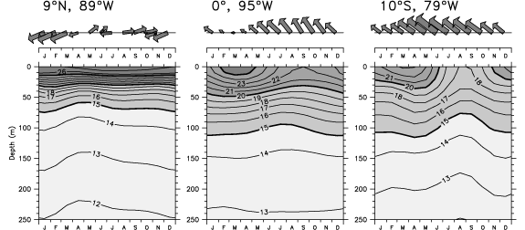
Fig. 9. Average annual cycle of wind stress vectors (top panels) and temperature (bottom panels) at the center of the Costa Rica Dome (9°N, 89°W; left), the equatorial cold tongue (0°W, 95°W; middle) and the Peru coastal upwelling (10°S, 79°W; right). Winds are the ERS scatterometer winds over 1991–2000, and both the length and thickness of the vectors increases with magnitude; the largest vector (June at the coast of Peru) has a magnitude of 5.8 N m. Temperatures are from the AOML XBT data set.

Fiedler's linear, wind-driven interpretation of the Costa Rica Dome annual cycle agrees with diagnoses made from much cruder data by Hofmann et al. (1981), but others have suggested that nonlinearities are also important. Umatani and Yamagata (1991) argued that cyclonic eddies produced near the coast by strong Papagayo winds "seed" the growing Costa Rica Dome and are an essential element of its formation. In the next section, we use a simple model consisting only of linear long Rossby waves to suggest that although the eastern tropical Pacific is rich with seasonal eddies, the low-frequency dynamics evolves principally according to a linear interpretation.

The Tehuantepec Bowl has a larger annual cycle amplitude than the Costa Rica Dome (Fig. 7), but has not been as well described in the literature. The bowl is nearly absent in boreal summer-fall, and grows as an isolated feature during boreal winter, with the 20 °C isotherm at least 10 m deeper than its surroundings. In spring, the thermocline trough at 15°N amplifies and appears to extend eastward as the bowl moves west, connecting the two. In the sequence of observed thermocline depth anomalies (left panels of Fig. 10), this can be seen as the deep thermocline centered at 13°N, 100°W in the JFM season that lengthens as a long trough to the west in April–May–June, then shoals (weakens) greatly in summer.

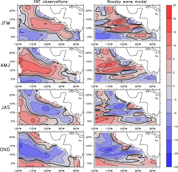
Fig. 10. Comparison of annual cycle anomalies of observed 20 °C depth (left panels) and the Rossby wave model solution (Section 4.2.1) (right panels), for four average seasons (indicated to the left of each row). The common color key is at right, with contour interval of 5 m. Positive values (red) indicate deep anomalies and negative values (blue) indicate shallow anomalies.

Winds and precipitation in the region between the equator and 10°N are strongly influenced by the large annual cycle of cold tongue SST, which is warmest in March and coolest in September (Mitchell and Wallace, 1992; Kessler et al., 1998). At minimum cold tongue SST, the temperature difference between the equator and the head of the Panama Bight is more than 6 °C, fostering the low-level southwesterly Choco jet (Poveda and Mesa, 2000; Amador et al., 2006), that feeds moisture to the west slopes of the Colombian Andes. The poleward coastal winds of the Choco jet are downwelling favorable, and Rodriguez-Rubio et al. (2003) use high-resolution satellite altimetry to argue that this produces a sea level high and anomalously anticyclonic circulation in the Bight during boreal summer-fall (though it remains unclear if the mean cyclonic gyre (Fig. 4) actually reverses or just weakens). Investigators are also beginning to explore the impact of SST variations driven by ocean dynamics on the precipitation fields on the region. Xie et al. (2005) showed that while the ITCZ stretches across the east Pacific warm pool in summer, persistently cooler SSTs above the Costa Rica Dome inhibit convection and produce a 500-km wide dry spot in the ITCZ at this time. Similarly, in winter the ITCZ moves south, drawing the Panama jet across the Isthmus and over the Pacific. Upwelling curl associated with the left (southeast) flank of this jet generates a cyclonic eddy in the Panama Bight and SST cooling in its center (Rodriguez-Rubio et al., 2003). As was seen to be the case when the ITCZ straddled the Costa Rica Dome in summer, a dry spot interrupts the convective precipitation over the Bight. The Tehuantepec jet does not have a corresponding effect because the large-scale precipitation in that region occurs in summer when the jet is inactive.

4.2.1. A Rossby wave model

Lacking data to diagnose the terms of the equations of motion directly, we examine solutions to simple models to evaluate their consistency with observations. If a simple model is able to reproduce the observed phenomena, there is no compelling justification for invoking more complex hypotheses. In situations where the simple model fails, it points to locations where other processes are active. The simplest first guess at the low-frequency, large-scale evolution of the off-equatorial thermocline is a model consisting only of long quasi-geostrophic Rossby waves forced by wind stress curl. This model adds elementary time dependence to the Sverdrup dynamics discussed in Section 4.1, allowing time-varying wind stress curl to pump the thermocline depth. It has been used by many investigators to interpret low-frequency variability in the tropical Pacific (Meyers, 1979; Kessler, 1990; Chen and Qiu, 2004).

Rossby waves are due to the latitudinal change in the local vertical component of the earth's rotation (zero at the equator, f/2 at the poles). Consider a symmetric hump of sea level, forced externally (say by downwelling wind stress curl). The geostrophic flow around the hump is westward on the equatorward side and eastward on the poleward side (like the Tehuantepec Bowl). However, because of the variation of f, flow on the equatorial side is stronger than that on the poleward side, thus more water is being transported westward than eastward. The result of this is to pile up water on the west side of the hump, and remove water from the east side. Therefore, the hump moves west from its initial position. That net transport is what makes a Rossby wave propagate west (and note that the westward propagation occurs equally well for a sea level depression, with the sense of the currents reversed). Because the difference in f across a hump of a given size is larger near the equator, the Rossby speed is much larger in the tropics.

The simple model has several potential weaknesses. By its neglect of velocity acceleration terms, the model excludes the near-equatorial waves that would be essential to study the region less than about ±3–4° latitude, but it has proven useful in the tropics (Kessler, 1990). By its neglect of nonlinear terms, the model excludes the advection of vorticity that has been shown to be important near the equatorial undercurrent (Kessler et al., 2003; and see Niiler, 2001 for estimates of these terms in the eastern tropical Pacific) and which may play a role near the narrow jet around the southeast corner of the Costa Rica Dome. The full range of effects of the nonlinear terms is not well understood; one likely consequence would be to change the "effective " and thereby the Rossby wave speed, by up to about ±50%.

The model can be written:

where h is the thermocline depth anomaly (positive down), is the wind stress and the density of seawater. The long Rossby wave speed is c = -c/f (c is the internal long gravity wave speed, f is the Coriolis parameter and its meridional derivative), and R is a damping timescale. Note that f is now allowed to vary with latitude. The two parameters to be chosen are the gravity wave speed c, which is estimated to be between 2 and 2.5 m s in the eastern tropical Pacific (Chelton et al., 1998), and the damping timescale R, typically taken to be (6–12 months) (Picaut et al., 1993). Here we choose c = 2 m s and R = (9 months); in fact the results are qualitatively insensitive to these choices within the reasonable ranges 1.75 m s ≤ c ≤ 3 m s and R ≤ (2 years). Additional realism could perhaps be achieved by choosing a different gravity speed c at each latitude, or by letting c be a function of longitude as well, but this did not seem necessary for the present purposes of making a first guess at the importance of the linear response to wind forcing. Solutions to the model encompass the local forcing by wind stress curl plus the subsequent westward propagation of any anomalies created.

Since long Rossby waves propagate non-dispersively due west, the wind-driven solution can be written separately at each latitude as an integral in x that sums the contributions of the wind forcing on the wave as it travels westward at speed c:

where h (x, t) is the interior wind-driven part of h. Note that Curl(/f ) in (2) is evaluated not at time t but at previous times looking back along the wave ray at speed c, that is, at times t - (x - x)/c. The lower limit of integration x is the longitude of the eastern boundary, and because the integration is westward, dx is negative.

Rossby waves can also radiate from the eastern boundary (for instance due to reflection of equatorial Kelvin waves), and these influences must be added to the interior solution (2):

where h is the damped effect of eastern boundary signals propagating to the interior. As done for the curl in (2), the value of h at the eastern boundary (h) is evaluated at previous times reflecting the lag for propagation from x to x.

The complete solution h to (1) is h from (2) plus h from (3); these are solved at each latitude independently and then combined. Here we use the average annual cycle of the ERS winds (see Appendix B) to force (2), and the eastern boundary value of observed 20 °C depth from the XBT data as h in (3). Solutions to (1) have also been found using other scatterometer winds (Quikscat) and from in situ wind products (FSU; see Appendix B) for various time periods, and the results are not strongly dependent on the wind data set used. In principle, a solution could be obtained entirely from the wind forcing, without the use of any ocean initialization along the boundary, using a basin-wide model to account for the generation of equatorial Kelvin waves, which may be forced by winds anywhere along the equator, or by western boundary reflections of Rossby waves. However, it is unclear how useful a single-baroclinic-mode model is over very long distances (e.g., Kessler and McCreary, 1993). In addition, observed near-coastal thermocline anomalies propagate poleward along the American coast very much slower than the coastal Kelvin waves a single-mode model would predict (Enfield and Allen, 1980; Chelton and Davis, 1982; Spillane et al., 1987; Pizarro et al., 2001; Strub and James, 2002c), so a purely wind-driven model clearly requires a realistic shelf structure and more complete baroclinicity (e.g., Clarke and Ahmed, 1999). Since we are interested here only in the eastern region and in the effects of wind stress curl, it seemed more appropriate to use the available information about the actual fluctuations along the boundary, rather than try to derive them from a model. In fact the boundary contribution to the total is small, except close to the coast, though it is noted that this contribution is essential in diagnosing changes in the coastal currents like the WMC, which depend on the offshore gradient.

The results of the Rossby model are compared to observed 20 °C depth anomalies in Fig. 10, for four average seasons. The solution can be thought of as a combination of westward-propagating Rossby waves forced by wind stress curl that seesaws annually across a nodal line at 8°N. The sum of the wave plus the local forcing appears as a generally southwestward phase propagation with wave crests approximately parallel to the Central American coast. (However, in fact the phase propagates purely westward at each latitude; the apparent meridional propagation occurs because the wind stress curl forcing oscillates so strongly out of phase across a nodal line at about 8°N, and the solution combines both local forcing and wave propagation.) In both the Rossby model and the observations, signals appear to originate as a thin region near the coast, grow and separate from the coast, and finally leave the region at the southwest corner. In general the model represents the magnitude and position of the observed thermocline signals reasonably well, though there is a sense that the model propagation is too slow at the northern edge and too fast at the southern (e.g., Kessler, 1990). It might be possible to improve this by varying the gravity wave speed c, but it seems useful to appreciate how well even the simplest type of model represents reality with minimum tuning.

A difference between model and observations is that the model solution depicts particular latitudes as having strong maxima, while the observations are smoother (Fig. 10). Since the model solutions are entirely independent at each latitude, its results are sensitive to narrow areas of strong wind stress curl, especially those associated with the mountain-gap wind jets (note the three positive maxima extending westward from the Tehuantepec, Papagayo and Panama jet outflow regions in the model JFM season). In reality, energetic eddies generated by the wind jets (but not represented in the linear model) produce horizontal mixing that blends latitudes together.

There is little indication of the features of the mean thermocline topography in the observed annual cycle anomalies (Fig. 10, left panels). No signatures of the mean ridges and troughs can be seen, nor of the Costa Rica Dome, nor of the regions of strong eddy activity. Instead the observations show a smooth southwestward propagation right across the strong thermocline topography and current shears. The good agreement with the model solution, which assumes a flat background thermocline (by the choice of a single value for c), with no eddy mixing, is evidence for the major role played by the linear response to wind forcing in the evolution of the annual cycle.

For the case of the Costa Rica Dome, the model correctly depicts the sequence of uplifting beginning at the coast early in the year, westward growth and separation in April–May–June, and strengthening of the ridge to the west of the dome in boreal summer-fall, as described by Fiedler (2002). Like the observations, the magnitude of thermocline depth variability at the dome is smaller than to its west; less than ±5 m compared to at least twice that further west (Fig. 10). The shoaling and extension of the dome into the Gulf of Tehuantepec in boreal fall is also evident in the linear model (lower right panels of Figs. 7 and 10). Similarly, the model correctly depicts the cutting-off of this bump in winter.

For the case of the NECC, the model shows that observed deepening along the 10°N ridge near 110°W in April–May–June that weakens the NECC (Fig. 7, lower left) is consistent with the wind forcing and Rossby wave propagation (Fig. 10, second row). In boreal fall the wind-forced Rossby wave produce the opposite anomalies (Fig. 10, bottom row), and the NECC strengthens (Fig. 7, lower right).

As noted above, it might well be thought that the climatological Tehuantepec Bowl simply reflects aliased sampling of the strong anticyclonic eddies that are due to the Tehuantepec winter wind jet (Willett et al., 2006). In that case one would expect that the linear Rossby wave model would not represent this feature very well. However, the model solution in fact captures the seasonal evolution of the bowl quite realistically, suggesting that its boreal winter-spring deepening is due to downwelling curl associated with the western side of the Tehuantepec wind jet, and the boreal summer shoaling is due to the upwelling curl from the eastern side of the jet that arrives later (Fig. 10, top and upper middle set of panels). The downwelling curl from Tehuantepec extends over the eastern part of the bowl (e.g., Fig. 1), so this is felt during immediately, during winter and soon after. By boreal spring, the downwelling Rossby wave extends past the west side of the bowl (Fig. 10, upper middle panels), establishing the connection to the basin-wide thermocline trough along 15°N (Fig. 7, lower left). However, the upwelling signal from the east side of the wind jet takes about 6 months to propagate to 105°W (at the relatively slow Rossby wave speed of 190 km month at 14°N), weakening the bowl in summer. Though the region just west of the Gulf of Tehuantepec that is strongly affected by the winter eddies might be expected to be a place where linear dynamics are least appropriate, the good correspondence of the simple model with reality shows that not to be the case.

Along the Central American coast, observed 20 °C depth anomalies suggest a poleward propagation with deep thermocline found at about 10°N in boreal winter, then moving along the southwest coast of Mexico in summer, arriving at the Gulf of California at the end of the year (Fig. 10, left panels). This is similar to the sequence shown from satellite altimetry by (Strub and James (2002b), see their Fig. 6), who show that this signal apparently stretches north to the coast of California. The mechanism of propagation remains unknown. Since the anomaly has a narrow offshore scale (a few hundred kilometers), the zonal gradient it produces results in poleward transport anomalies along the coast of Mexico (strengthening the WMC) during boreal summer and fall.

We can conclude from the Rossby model comparisons that these simple dynamics gives a good first-order picture of the annual cycle evolution in the northeastern tropical Pacific. The large-scale features of the regional evolution are principally explained by a linear ocean response to wind forcing, despite the evident possibilities of a fundamental role for the energetic eddies and their more complex dynamics. That means, for example, that one should not see the annual cycle of the Costa Rica Dome as an isolated phenomenon. Instead, the westward growth of the dome and its separation from the coast reflect the passage of the regional-scale Rossby wave seen in Fig. 10. Discrepancies are found in the model wave being broken into specific latitude bands while the observations are smoothly connected across latitudes; presumably this would be improved by a model that additionally allowed communication across latitudes by horizontal eddy mixing, as occurs in the ocean.

4.3. Eastern equatorial Pacific: mean and annual cycle

Relatively much less is known about the circulation in the far eastern than in the central equatorial Pacific, and a full picture of the currents and their interconnections is yet to be accomplished. In the central Pacific, where the winds are nearly zonal, the circulation is dominated by a westward surface SEC, with an eastward EUC in the thermocline (Fig. 6, top); Ekman divergence transports surface water away from the equator in both hemispheres, and consequently produces strong equatorial upwelling. In the east several of these elements are modified by weaker trade winds that also have a strong southerly component (Fig. 1). In addition, the zonal thermocline slope that balances equatorial easterlies (McPhaden and Taft, 1988) means that the thermocline and EUC rise much closer to the surface towards the east, trapping a complex mix of processes within a thin layer (Fig. 6). Upwelling increasingly drains water and momentum from upper layers of the EUC as it flows east.

Drifter tracks (Fig. 4; and see Reverdin et al., 1994) suggest that the near-surface SEC is weak east of about 85°W, and rapidly gains speed as it flows west. This was described by Wyrtki (1966), who correctly interpreted the increase as a sign that the SEC was gaining mass from the decelerating EUC below (as noted in Section 2 the role of the vertical circulation was not understood until later). Although there are no data to allow an estimate of the transport of the SEC east of 95°W, where it appears to be quite small (Fig. 6, bottom, and Fig. 4), the Johnson ADCP data (Appendix C.1) resolves SEC transport on the 15° longitude spacing of the TAO lines, beginning at 95°W. SEC transport above 200 m within 6°S–6°N at 95°W is about 12 Sv, increasing to about 35 Sv by 140°W, consistent with this interpretation.

Both the drifters (Fig. 4) and the ADCP data (Fig. 6) show that the SEC is split into two lobes, and is thin and weak on the equator, where the EUC surfaces or nearly so. Just south of the equator from the Galapagos to about 110°Wthe mean surface zonal flow is near zero, and a strong southward divergence from the equator is seen (Fig. 4). Although the drifter population is smaller in this region (because the drifters diverge rapidly from the equator), sampling problems do not appear to explain this unexpected feature. The same weak surface current appears in the Johnson et al. (2002) ADCP data and is consistent with the very small mean surface zonal currents measured by the TAO mooring at 0°W, 110°W (Kessler et al., 1998). The splitting of the SEC has been attributed to upwelling of eastward momentum from the EUC, and interpreted as an important nonlinear effect of easterly equatorial winds (Philander and Pacanowski, 1980; McPhaden, 1981), but weaker easterlies over the cold tongue, caused by atmospheric boundary layer effects of the cold SST (Chelton et al., 2001), may also contribute.

The EUC surfaces during boreal spring, changing the near-surface flow at 0°W, 110°W to eastward at more than 20 cm s during the average April and May (Kessler et al., 1998; Yu and McPhaden, 1999a,b); this reversal reduces the annual mean zonal current at 110°W to near zero. While the eastern EUC shoaling occurs when local easterly winds are weakest, this is part of a basinwide phenomenon that begins in the far east in March, and reaches the dateline by about August (Reverdin et al., 1994; Yu and McPhaden, 1999b; Johnson et al., 2002); it is forced by the westward-propagating annual cycle of zonal wind along the equator producing a mixture of equatorial Kelvin and long Rossby wave modes (Yu and McPhaden, 1999b; Wang et al., 2000). Wind-forced ocean models show this signal clearly (e.g., Yu et al., 1997; Kessler et al., 1998). Because the mean EUC is much shallower in the east, it is only here that an actual reversal of the surface westward flow is seen: the surface current along the equator is eastward from about 140°W to at least 95°W during boreal spring (Johnson et al., 2002). It is worth noting that the seasonal cycle has an unexplained low-frequency modulation and has been observed to change substantially in amplitude in different decades (Gu et al., 1998).

The fact that the weakest SEC is found just south of the equator (Figs. 4 and 6, bottom) is consistent with the meridional circulation induced by southerly cross-equatorial winds (Fig. 1); note that the coldest SST is also south of the equator (Fiedler and Talley, 2006). These winds drive a vertical circulation cell that is downwind (northward) at the surface and upwind in the thermocline, with enhanced upwelling south of the equator (Philander and Delecluse, 1983; Mitchell and Wallace, 1992; Kessler et al., 1998). This cell therefore advects westward wind-input momentum northward across the equator, and upwells eastward momentum from the EUC at about 1–2°S, contributing to the asymmetric pattern seen in Fig. 4. (Although the northward surface velocity predicted by this theory is not apparent in Fig. 4, it is seen in the TAO moored velocity at 110°W.)

A comprehensive examination of hydrographic data by Lukas (1986) showed that high-salinity, high-oxygen water flowing eastward in the EUC can be detected all the way to the coast of Ecuador and Peru (Fiedler and Talley, 2006), indicating that at least the deeper layers of the EUC continue further east than the Galapagos. Some model results suggest that the physical blocking of the EUC by the Galapagos Islands leads to a surge of upwelling west of the archipelago, abruptly draining off its upper layers (Eden and Timmermann, 2004), but the salinity and oxygen properties imply that the lower EUC feeds the Peru Undercurrent and becomes a source of the Peru upwelling (Brink et al., 1983). Toggweiler et al. (1991) confirmed Lukas' result using C measurements from coral heads. They suggested that low C water originates in the subantarctic region of the southwest Pacific, flows north to enter the lower reaches of the EUC, and populates the east Pacific thermostad to eventually upwell off Peru. Note that Peruvian coastal upwelling is strongly seasonal, and appears to reach far into the thermocline and below (Fig. 9, right), consistent with this being the destination of thermostad water. Steger et al. (1998) found evidence of the EUC splitting around the Galapagos with the main branch flowing to its south. On the other hand, the only published measurement of the EUC in the far east was made using an underway ADCP profiler on WOCE cruise P19 along 86°W in March 1993 (Tsuchiya and Talley, 1998); this showed what appears to be a strong EUC (70 cm s) centered just north of the equator at 70 m depth. However, this period was during a weak El Niño that produced several Kelvin wave pulses of eastward equatorial currents that were observed further west around this time (Kessler and McPhaden, 1995b), so the single P19 section may very well not represent the mean. In addition to Lukas' water property evidence, it should be suspected that the EUC would be found south of the equator because of the meridional circulation cell mentioned above in connection with the SEC.

Dynamically, it is not clear why there should be an EUC east of the Galapagos, because the usual understanding of the undercurrent suggests that it is driven by the zonal pressure gradient, which itself is due to the mean easterly winds characteristic of the central Pacific. East of about 90°W, the zonal winds are very weak or westerly (Fig. 1), so according to linear dynamical ideas there should be no pressure gradient or EUC. (Note that the weak SEC in this region (Fig. 4) is consistent with the weak zonal winds). In fact, the integrated zonal pressure gradient calculated from the AOML XBT data relative to 450 m is reversed in the far east. This difficulty was recognized by Roden as early as 1962. A possible piece of the answer was proposed by Kessler et al. (2003), who used an ocean GCM to show that eastward advection of cyclonic relative vorticity on the flanks of the EUC strengthened both the EUC and SEC branches well east of where an eastward undercurrent would be expected from linear dynamics, which is consistent with observations of these currents at 140°W and 110°W. While they had no data to compare with the far eastern Pacific mode results, this nonlinear mechanism would act to produce an EUC in the far east even without a pressure gradient to drive it.

Although most of the EUC appears to flow all the way to the Peru coast in the thermocline, there is also substantial downstream loss of EUC water to the surface layer by upwelling, and the destination of this water remains in question. Presumably the surface flow combines a diverse and hard-to-quantify set of competing processes acting within the thin upper layer, including poleward Ekman divergence, westward and northward directly wind-driven currents, and the surfacing eastward EUC. An inverse calculation using the hydrographic data compilation of Johnson et al. (2002) suggested that about 10 Sv of equatorial water above the thermocline (including water upwelled from the upper layers of the EUC) is transported northward in the surface layer (Sloyan et al., 2003). They argued that this was one of the pathways by which intermediate water entering the South Pacific was transported to the northern hemisphere (and eventually to the Indonesian Throughflow). By contrast, Blanke and Raynaud (1997) diagnosed Lagrangian trajectories in an ocean GCM and came to the opposite conclusion: that most of the water upwelled from the EUC in the east exited towards the south. Clearly this issue remains unsettled.

The role of the distinctive equatorial circulation in producing the vertical and horizontal exchanges that maintain the east Pacific cold tongue and the sharp SST front along about 2°N has been the subject of a great deal of research over 50 years (e.g., Cromwell, 1953). Most of this work has concerned the central Pacific upwelling zone, but many of these processes are relevant to at least the part of the eastern equatorial Pacific west of the Galapagos, and the major points will be reviewed briefly here. The temperature balance is generally thought to be among equatorial upwelling and vertical mixing, meridional mixing across the SST front, and surface heating. Perhaps surprisingly, zonal advection may be less important. The continuous band of cool SST connecting the coast of Peru with the equatorial cold tongue suggests advection of coastal water out along the equator. However, the southwestward surface currents west of Peru (Fig. 4), consistent with the Ekman drift implied by the mean winds (Fig. 1), do not support such a hypothesis, nor is there evidence of continuous flow connecting the coastal and offshore regions (Fig. 4). Some model experiments also contradict this idea. Kessler et al. (1998) put a wall extending 700 km westward from the Ecuadorian coast at 4°S in an ocean GCM and found little difference in SST along the equator west of the Galapagos, either in the mean or in the annual cycle. Note that coolest SST along the equator occurs less than a month after that at the coast (Fig. 9), probably too fast to be due to advection. Instead, the thermal structure changes in both regions are consistent with local wind-driven upwelling; SST cooling is associated with thermocline uplift that occurs in phase with increases of the local winds. A contrasting view was given by Swenson and Hansen (1999), who used drifter data to estimate that advection had an non-negligible influence on the heat budget on the equator, and hypothesized that this was partly due to transport from the coast. It is also thought that during El Niño events, zonal advection from the west can be a significant contribution to SST warming, at least in the central Pacific (Picaut et al., 1996).

Numerous attempts to measure upwelling velocity have been based on finding the divergence of measured horizontal currents; e.g., Weisberg and Qiao (2000) used moored current meters, Johnson et al. (2001) used repeated shipboard ADCP sections, and Hansen and Paul (1987) used surface drifter currents. Indirect methods have been based on divergence of geostrophic and Ekman transports around large boxes spanning the cold tongue (Wyrtki, 1981; Bryden and Brady, 1985; Meinen et al., 2001). All these studies have estimated upwelling velocities on the order of a few m day, with total vertical transport of 30–50 Sv over the east-central Pacific, though the spatial pattern of upwelling (whether broad and relatively slow, or narrow and correspondingly fast) remains unknown. There is also little agreement on the depth to which upwelling reaches as it works against the stratification of the upper thermocline. Cross-isopycnal transport requires either heating from above (for example through penetrating radiation) or turbulent mixing, which is just beginning to be understood (see, e.g., Lien et al., 1995). While upwelling transport is due to the local Ekman divergence, its effect on SST and nutrients in the upper layer depends very much on the background stratification, which is modulated by basinscale conditions. Despite the many uncertainties, there is no doubt that upwelling is an order(1) term in the heat and mass balance of the equatorial Pacific, both in the mean and in its seasonal and interannual variability. Since upwelling is so important but at the same time impossible to measure directly, attention has been given to consistency checks that compare the heat fluxes due to upwelling to other elements of the heat balance (Wang and McPhaden, 1999, 2000).

Mixing across the SST front north of the equator opposes the cooling due to upwelling. This mixing primarily takes the form of tropical instability waves (TIW), which are due to the shears between the eastward EUC and NECC and the westward SEC (Fig. 6), (Philander, 1978; Willett et al., 2006). It was first thought that the NECC-SEC shear was the key element, but some investigators now argue that the EUC-SEC shear is important as well (Yu et al., 1995; Chelton et al., 2003), and this question remains controversial. The TIW distort the front into cusp-like shapes that are easily seen in satellite imagery (Legeckis, 1977; Chelton et al., 2000; Chelton et al., 2001), and result in a substantial equatorward heat transport by mixing across the front, as tongues of warm water move south and cool water move north. Hansen and Paul (1987) and Bryden and Brady (1989) estimated this heat flux as comparable to that due to upwelling, and other observational balances and model experiments agree.

The tendency to compensation between upwelling cooling and TIW warming occurs in the annual cycle as well. As winds strengthen in the second half of the year (Fig. 9), the SEC and NECC both strengthen (see Section 4.2 and Fig. 7), as does equatorial upwelling. These tendencies cool the equator and warm the region north of the SST front, increasing the SST gradient as well as strengthening the shear that drives the TIW and thereby produces stronger mixing. Therefore, during June–December, opposing SST tendencies are generated and the net effect of these ocean fluctuations on SST is smaller than might be assumed from the upwelling increase alone (Enfield, 1986; Kessler et al., 1998; Swenson and Hansen, 1999). During El Niño events, by contrast, surface and local vertical fluxes are dominant (see next section).

Although the sun crosses the equator twice a year, in March and September, only an annual cycle is observed in SST, which is coldest in September (Mitchell and Wallace, 1992; Kessler et al., 1998; Fiedler and Talley, 2006). A major factor constraining SST to a simple annual cycle is the cooling due to equatorial upwelling. The entire thermocline rises about 20 m during June–September (Fig. 9, middle), bringing cool water within reach of mixing by the stronger winds. Another is the variations of the extensive stratus decks that cover the cool-water part of the eastern tropical Pacific, south of the SST front (Klein and Hartmann, 1993), that are at least partly driven by annual variations of the subtropical high pressure zones. The interaction of stratus clouds and cool SST comprises a positive feedback, since cool SST encourages the formation of stratus that reduces the September solar cycle maximum and therefore reinforces the SST anomalies. A similar situation prevails in the eastern Atlantic. Disentangling the diverse ocean-atmosphere influences on the eastern tropical oceans remains a central climate problem of the region that is just beginning to be attacked (Cronin et al., 2002).

4.4. El Niño variations

Although the episodic warming off the Peru coast had been known and named El Niño since the 1890s (Philander, 1990), its connection to the planetary-scale "Southern Oscillation" was only beginning to be understood with the pioneering work of Bjerknes (1961, 1972). The mechanism of coastal warming continued to be assumed local until Wyrtki (1974a, 1975a) used island and coastal sea level time series to establish that mid-Pacific westerly wind anomalies generated downwelling Kelvin waves that deepened the eastern thermocline and allowed warming to occur, independent of the local winds. The key to this insight was the realization that coastal winds during El Niño events were usually upwelling-favorable, and thus could not produce the observed warming (Fig. 11). Noting the strong alongshore winds during the 1964–1965 El Niño, Wyrtki (1975a) commented "Consequently, one must abandon the idea that winds off Peru are abnormally weak during the periods of El Niño, and one must search for other ways to explain this phenomenon". The extreme SST, wind and rainfall anomalies produced by the El Niño of 1982–1983 spurred a major effort that continues to the present to observe and understand the ENSO (El Niño-Southern Oscillation) phenomenon (see, e.g., McPhaden et al., 1998; Wallace et al., 1998; and Neelin et al., 1998, for reviews of this effort, and Wang and Fiedler, 2006, for a review of recent theories). Today we know that El Niño events begin in the western Pacific and spread eastward, with the Peru coastal warming one of the final signatures. During most El Niño events, winds over the eastern Pacific change late in the event, if at all, and the SST warming that occurs in the east is primarily remotely forced (Huyer et al., 1991; Cronin and Kessler, 2002; Carr et al., 2002). As Wyrtki realized, the drastic changes in thermocline depth and currents occur as the result of wind-forced variability carried to the east by equatorial Kelvin waves (Spillane et al., 1987; Enfield, 1987; Kessler and McPhaden, 1995b). Westerly wind anomalies over the western and central Pacific flatten the equatorial thermocline across the basin, and at the same time greatly weaken the SEC (Fiedler et al., 1992; Kessler and McPhaden, 1995a; Lagerloef et al., 1999; McPhaden, 1999; Wang and McPhaden, 2000; Bonjean and Lagerloef, 2002). Although the SEC is partly frictionally driven by the trade winds, it can weaken substantially even in the absence of local wind changes because the deepening equatorial thermocline depresses the upward bulge that in normal conditions produces westward geostrophic shear above the EUC (e.g., Fig. 6). Thus eastward current anomalies span the equator, and advection appears to be a significant part of the El Niño warming in the west-central Pacific (Kessler and McPhaden, 1995a; Ralph et al., 1997), although it is probably not the case that warm west Pacific water is carried all the way across the basin (Picaut et al., 1996; Bonjean, 2001). In the east, the most important warming influence appears to be that the deeper thermocline allows local surface fluxes to heat the surface layer (Kessler and McPhaden, 1995a; Vialard et al., 2001; Cronin and Kessler, 2002) as the source of cool upwelled water is cut off (although upwelling within the thick warm layer may still be occurring under near-normal easterly trade winds). A positive feedback occurs because warmer SST tends to inhibit the formation of the usual east Pacific stratus decks, thereby allowing further warming. Although warmest actual SSTs tend to occur in January–March of the year following the largest El Niño wind anomalies, warm SST and eastward zonal current anomalies have usually peaked in the previous September; thus El Niño appears in the east as a suppression of the cold phase of the annual cycle. It is not known why El Niño events are phase-locked to the annual cycle in this way (Wang and Fiedler, 2006).

Fig. 11. The Southern Oscillation Index (top) and interannual wind stress anomalies along the coast of Peru (bottom). Interannual anomalies are defined as the 11-month running mean of anomalies from the average annual cycle. Shading shows stress anomaly magnitude, with shading levels every 0.1 N m; lighter shades show weaker than normal winds, with a contour drawn at zero. The scale vector is at lower left. Negative SOI corresponds to El Nino conditions.

Most studies of ENSO have concentrated on the equatorial strip; there is far less information to diagnose interannual variability in the eastern Pacific warm pool region, except for SST time series, for which instrumental records with sufficient spatial resolution to examine detailed features extend back to 1981 (Appendix C.2). The XBT data used in this study (Appendix A.1) were taken during the period 1979–1996, but contain few places with sampling sufficient to produce interannual timeseries. Because of the paucity of subsurface data, Fiedler (2002) cited the results of a numerical model forced with observed winds to comment briefly on interannual variations of the Costa Rica Dome during 1980–2000 (he noted that it was weak or absent in El Niño years and was apparently stronger in the one La Niña year simulated by the model). Barberan et al. (1984) compared the results of two CTD surveys across the dome during relatively normal conditions in 1979 versus early in the El Niño event of 1982, finding a large increase in isotherm depths and implied poleward speeds along the coast but relatively small anomalies in the center of the dome. Other data sets that have been used to study interannual variability in the tropical Pacific include island sea level records (Wyrtki, 1974b, 1979), but these provide less detail on the oceanic conditions in the east because the only long records are along the coast. For these reasons, some studies of interannual variations in the northeastern tropical Pacific have relied on correlating basin-scale modes with coastal time series (Baumgartner and Christensen, 1985). However, diagnosing the mechanisms of variability requires analysis of the offshore spatial patterns of currents and thermal structure.

The lengthening time series from the Topex altimeter (Appendix C.3) have been used in several comprehensive descriptions of eastern Pacific annual and interannual variability (Strub and James, 2002b,c; Carr et al., 2002). The Topex instrument gives a good picture of the evolution of the region since its launch in 1992, sampling at least the El Niño of 1997–1998 and the change to La Niña conditions following that event, and we will use its spatial variability pattern to interpret interannual SST variability. Of course it must be kept in mind that statistics of the Topex variations are dominated by the very large signals of 1997–1998 (Strub and James, 2002a), and are not necessarily typical of El Niño events over the long term.

A description of the spatial pattern of interannual variability of both the Topex sea level and SST is constructed by correlating interannual variability across the region with that at 0°W, 95°W (Fig. 12), which is a good index for ENSO. For SST, correlations among the interannually smoothed 20-year time series have about 15 degrees of freedom, which means that correlation values greater than about 0.5 are significantly different from zero at the 95% level, indicated by gray shading in Fig. 12. For sea level, there are fewer degrees of freedom, and correlations are significant above about 0.7. In either case, significant correlations indicate a close correspondence of interannual variations all along the equator and spreading poleward in a narrow region along the American coast. This is a classic signature of El Niño, in which deep thermocline anomalies (equivalently high sea level), accompanied by warm SSTs, propagate eastward along the equator as Kelvin waves, then poleward along the Americas. One might consider these two maps to represent anomalies of SST and sea level at the height of a warm event. It is noted that a correlation map similar to that in Fig. 12 (top) was found from the Kaplan et al. (1998) SST record that spans more than 100 years.

Fig. 12. Correlations of interannually smoothed quantities with the same quantity at 0°W, 95°W. Top: SST from the Reynolds SST product (1981–2005). Bottom: sea level from the Topex/Jason altimeter (1993–2005). Interannual anomalies are defined as the 11-month running mean of anomalies from the average annual cycle. Shading indicates correlations significant at the 95% level (see text).

High interannual SST correlations extend to 8–10°N east of 120°W, while sea level correlations are high only to 6–7°N (Fig. 12). As mentioned above, SST changes within the eastern equatorial region are primarily due to vertical processes associated with the deepening thermocline, however the correlation patterns suggest that the meridional height gradient on the northern flank of the sea level anomaly drives eastward geostrophic currents that warm the extra-equatorial region by advection. This is consistent with previously observed increases in the flow of the NECC, and corresponding weakness or reversal of the SEC at 5–10°S, in the central Pacific during El Niños (Kessler and Taft, 1987; Kessler and McPhaden, 1995a), which are also associated with the increased depth of the cross-equatorial thermocline at the height of the warm event. Indeed, when sea level anomalies from Topex during late 1997 are added to the seasonal XBT dynamic heights (Fig. 7), the surface height gradient across the NECC is approximately doubled, all the way up around the southern limb of the Costa Rica Dome, as is suggested by Fig. 12 (bottom). Further, since the sea level anomalies follow the coast narrowly, the Costa Rica Coastal Current is also greatly enhanced. However, this flow continues north along the coast rather than circling around the dome, and thus should not be seen as a strengthening of the dome itself, but due instead to narrow thermocline deepening along the coast, with its offshore scale determined principally by the width of coastal Kelvin waves. Thermocline anomalies in the dome are poorly correlated with equatorial anomalies (note the 0.9 contour looping around the dome Fig. 12, bottom), and the center of the Costa Rica Dome deepens only slightly during El Niño events (Barberan et al., 1984; Fiedler, 2002).

The coastal El Niño signals are frequently noted as surges of poleward flow that can continue all the way to Alaska and Chile at timescales from intraseasonal to interannual, most commonly during the boreal winter season (Chelton and Davis, 1982; Spillane et al., 1987; Hormazabal et al., 2001; Strub and James, 2002c,a; Carr et al., 2002; Hormazabal et al., 2002). As noted in Section 4.1, several investigators have shown evidence of increased penetration of tropical water to the mouth of the Gulf of California associated with El Niño events (Baumgartner and Christensen, 1985; Filonov and Tereshchenko, 1999; Lavín et al., 2003), consistent with Fig. 12, associated with these surges. Comparable low-frequency pulses of the Peru-Chile Undercurrent driven by El Niño-generated Kelvin waves were described by Pizarro et al. (2002).

We noted above that the occurrence of upwelling-favorable winds along the Peru coast during El Niño events (Fig. 11) led Wyrtki (1975a) to realize that the quintessential signature of coastal warming must be remotely forced and hence that El Niño was a connected basinwide phenomenon. While the coupled dynamics that produce the coastal wind anomalies has not been diagnosed in the literature, it is consistent with an atmospheric boundary layer response to heating by SST. El Niño SST anomalies are largest from the equator to about 5°S along the coast, which makes the anomalous SST gradient northward during warm events, fostering equatorward winds at Peruvian latitudes as observed (Fig. 11). This would be an example of winds forcing the ocean in one place, oceanic Kelvin waves carrying the signal in thermocline depth across thousands of kilometers, thus changing the SST remotely, which then feeds back to modify the winds in the distant location.

5. Remaining questions

The central remaining physical oceanographic problem of the eastern tropical Pacific is the three-dimensional interconnection among the zonal currents of mid-Pacific as they impinge on, or depart from, the American coast. Wyrtki realized this early on, and drew a schematic (Fig. 5a) that is not so different than one drawn today (Fig. 5b), except in added detail; however that is mostly a statement that we are still unable to produce a quantitatively realistic picture. The interconnections among the EUC, SEC and Peru upwelling remain difficult to diagnose with presently available data, while model descriptions appear to be highly dependent on the resolutions and physical parameterizations in the various models.

We know, as Wyrtki did, that some of the EUC upwells into the SEC, while another part continues southeastward at thermocline depth to feed the Peru upwelling (Roden, 1962; Lukas, 1986) but are not much further along in putting numbers to this than was possible in 1966 (see Sloyan et al., 2003, for an estimate from an inverse calculation). In general the eastern origin of the SEC remains almost as shrouded in mystery as it was in Wyrtki's time. How much of the SEC comes from equatorial upwelling, how much from the NECC, and how much from the Peru coast? We can assume that this division varies both seasonally and interannually, but can barely speculate on the answers. A further puzzle concerns the very thick westward flows on both sides of the EUC, that appear to be deep extensions of the SEC branches (Fig. 6, middle panel). (Although these appear only weakly in the 90°W section (Fig. 6, bottom), they exist down to the 900 m reference level at both 110°W and 90°W in this data set.) Rowe et al. (2000) hypothesized that these could be the westward limb of deep cyclonic gyres fed by the two Tsuchiya Jets. This has been difficult to confirm with the very sparse data coverage available.

The vertical circulation in the eastern tropical Pacific has local and basin-scale origins and consequences. The large-scale winds constrain the thermocline to tilt down to the west and be shallowest along the coast of the Americas (Fig. 9 of Fiedler and Talley, 2006). Local regions of upwelling-favorable winds (the Central American wind jets and alongshore winds on the coast of South America) can therefore open a window through which thermocline (and subthermocline) water can reach the surface and interact with the atmosphere. Although it has been known for centuries that the upwelled water is nutrient-rich and thus has tremendous economic and ecological importance, the mechanisms that control and produce variability of east Pacific upwelling remain not well diagnosed. The processes occurring off Central America have been discussed in several papers as reviewed in Sections 4.1 and 4.2 above, but upwelling along the Peru-Chile coast poses many unanswered questions. In particular, the depth of upwelling's reach, and the dependence of this depth on the background stratification, is poorly understood. Since the stratification can change in response to either Kelvin wave propagation or water mass advection from the equator, while the upwelling velocity itself is driven by local winds, variability of SST due to upwelling is produced by a mix of local and remote influences that have not been clearly identified or quantified.

The basin-scale impacts of coastal upwelling are even less well understood. The continuity of low SST from the coast of South America to the equatorial cold tongue, both in the mean and annual cycle (see, for example, Fig. 4 of Fiedler and Talley, 2006) might be taken to indicate that cold upwelled water advects from the coast out along the equator. This would provide an oceanic connection between the two cold regions and a mechanism by which equatorial SST, with its planetary impacts through the ENSO cycle, could be influenced by South American coastal wind variability. However, as noted in Section 4.3 above, this is by no means proven, and some evidence indicates that the Peru and equatorial upwelling regions are separately driven by their regional winds. In this case there might still be a connection through an atmospheric bridge.

A potentially important impact that is beginning to be investigated is the relation between South American coastal upwelling and the persistent stratocumulus cloud decks that are a principal feature of the climate of a very large region of the southeast Pacific (Klein and Hartmann, 1993; Yu and Mechoso, 1999; Kollias et al., 2004; Xu et al., 2005). These cloud decks have been one of the worst-simulated aspects of global coupled climate models, and are thought to be a major contribution to fundamental biases that confuse the interpretation of climate change (Davey et al., 2002; Bretherton et al., 2004). We noted in Section 4.3 above that the shading of the ocean due to stratus cools SST, inducing a positive feedback by chilling the lower atmospheric boundary layer, which fosters the continuation and growth of the stratus. Thus one could hypothesize that the initial trigger is the coastal upwelling, which, though it has a narrow scale of perhaps 50–100 km, could cool the atmosphere in the region immediately adjacent to the coast. Since upwelling is due to offshore Ekman advection of surface water, this would tend to push the cold SST offshore, increasing the area of cloud coverage and potentially driving this whole system. However, there are other influences that foster the stratus decks, especially the general subsidence of the atmosphere under the subtropical highs; recent diagnoses have suggested that this is episodically amplified by atmospheric communication from convection over interior South America (Colbo and Weller, submitted for publication). It has proven difficult, however, to quantify the various influences on the delicate balances that produce the stratus decks, and a field study to study these processes is being planned (VOCALS Scientific Working Group, 2005).

As mentioned in Section 4.3, water property evidence implies that EUC and much of the thermostad water below it originates in the southwest Pacific (see Fiedler and Talley, 2006). The Indonesian Throughflow represents a transport of approximately 10–15 Sv; this amount of intermediate water entering the South Pacific from the Southern Ocean leaves the North Pacific as surface water. Thus the water mass must both have its potential vorticity modified to change hemispheres and it must be upwelled, so that this transport can be effected. Both the water mass transformation and upwelling presumably occur in the eastern tropical Pacific, as some combination of equatorial, Costa Rica Dome and Peru-Chile upwelling. This suggests that these distinctive features of the eastern tropical Pacific play a material part in the global ocean circulation.

Acknowledgement

I thank Paul Fiedler and Miguel Lavín for encouraging me to take on this review, and for many helpful comments during its preparation. David Enfield, Maria Donoso and Pilar Cornejo at NOAA/AOML kindly provided their quality-controlled XBT data that is the foundation of this study. Antonio Badan-Dangon prodded me to open my mind concerning the CRCC. Emilio Beier carefully read the manuscript and saved me from some embarrassing errors. My understanding of the development of ideas about the circulation of the eastern tropical Pacific was greatly aided by three scientists who were early and ongoing contributors to the exploration and interpretation of the region: Gunnar Roden, Bruce Taft and Warren Wooster. They generously shared stories, analyses and documents, for which I am very grateful. This is a contribution to the scientific agenda of the Eastern Pacific Consortium of the InterAmerican Institute for Global Change Research. Support was also provided by the Protected Resources Division of NOAA Fisheries, Southwest Fisheries Science Center.

Appendix A. Data sources and preparation

A.1. A XBT data

The principal thermal data set used in this study is the historical XBT compilation of Donoso et al. (1994), which will be referred to here as the "AOML XBT data". These profiles originated from earlier compilations produced principally by the National Ocean Data Center, the Joint Environmental Data Center at Scripps, and the Global Subsurface Data Center in Brest, France. A total of 36,185 profiles were available within 15°S–25°N, and from 120°W to the American coast; as is typical of volunteer observing ship data, the profiles were primarily organized along the major shipping routes. The main concentration of profiles were taken during 1979–1992, with smaller numbers after that date. Donoso et al. (1994) describe the objective and subjective quality control procedures used to flag questionable observations and produce a research-quality data set. Only data points they found to be acceptable were used in this study.

The irregularly distributed profiles were mapped to a regular 1° latitude by 1° longitude by 10 m by climatological-month grid in two steps. First, the temperature data in each individual profile were linearly interpolated to 10 m depth intervals from the surface to 450 m (on average, each profile had about 41 samples in the upper 450 m). Second, in a separate calculation at each 10 m level z, the irregularly spaced temperatures were mapped onto the (x, y, z, t) grid using a Gaussian-weighted three-dimensional mapping (Kessler and McCreary, 1993), with scales of 2° longitude, 1° latitude and 2 months. The region of influence of each observation was limited to where its weighting was greater than e, that is, to twice the scale distance from the center of each gridbox. Only the month was considered in the gridding, not the year, to produce a climatological average annual cycle. These data were previously used in a study of the mean circulation (Kessler, 2002), and the same gridding procedure was used here.

Although some earlier XBT-based climatologies of the entire tropical Pacific used coarser grid spacings [e.g., Kessler, 1990, who mapped onto a 5° longitude by 2° latitude grid], the short spatial scales of the phenomena of interest in this region required higher resolution, and the profile distribution in the new compilation was dense enough to justify a 1° × 1° spacing. Each 1° × 1° gridbox contained, on average, more than 24 profiles during the year, spread over an average of 7.4 months. The gridded temperature climatology was checked by comparison against other sources, including the Reynolds SST (Reynolds and Smith, 1994) and time series from the TAO mooring array (McPhaden et al., 1998).

Dynamic height relative to 300 or 450 m reference levels was found from the gridded temperatures via a mean T-S relation constructed from the Levitus et al. (1994) atlas, and geostrophic currents were found from centered differences of the dynamic heights.

An additional meridional section at 125°W, shown in Fig. 6, was constructed from the XBT data compilation of Kessler (1990). These data partly overlap the AOML XBT compilation, but extend further west. Quality control and gridding is described by Kessler (1990); of note is that the lesser data density required a coarser gridding as mentioned above. Along the 125°W section shown, 50–150 profiles were found in each 2° latitude by 5° longitude box, roughly half as dense than the AOML data.

Appendix B. Scatterometer wind data

Winds are used in this study to estimate Ekman pumping and to force a Rossby wave model (Section 4.2.1). Since the winds in this region are known to have small spatial and temporal scales (Chelton et al., 2000a), especially in the case of the mountain-gap wind jets that are found to have great importance, and because these calculations require spatial derivatives of the winds, excellent sampling is a necessity. This points to the utility of satellite scatterometer winds that can resolve the wind jets better than any in situ or present-generation reanalysis wind product (Schlax et al., 2001). The Quikscat satellite carrying a Seawinds scatterometer (referred to here as Quikscat) was launched in June 1999 and its operational products became available in late July 1999. The satellite circles the earth in a 4-day repeat, sun-synchronous orbit with a spacing of 6.3° at the equator, sampling a 1600-km wide swath centered on its ground track. The first three years of Quikscat wind stresses were obtained on a 1° × 1° grid from the web site of Center for Ocean-Atmosphere Prediction Studies (http://www.coaps.fsu.edu/scatterometry/) at Florida State University (FSU), and used to represent the mean winds.

The European Research Satellite (ERS) was launched in July 1991, and its nearly identical follow-on mission was launched in April 1995 and remains in operation (but a gyroscope failed in January 2001, degrading the data). Data used here include the period August 1991 through December 2000. ERS data are processed onto a 1° × 1° monthly grid by the Centre ERS d'Archivage et de Traitement (CERSAT), at IFREMER, Plouzan'e (France), and are available at http://www.ifremer.fr/cersat. The ERS sampling is not as good as Quikscat, with a 500-km wide swath and 35-day repeat cycle. However, the nearly 10 year record is more suitable for estimating the average annual cycle, and the ERS winds are used here to force a Rossby wave model (Section 4.2.1). Extensive comparison has been made between the two scatterometer products, and also with in situ wind products (the widely used Florida State University (FSU) product, which spans 40 years (Stricherz et al., 1992)). All these winds show quite a consistent picture in the eastern tropical Pacific; the differences are essentially that Quikscat gives greater spatial detail than ERS, which in turn gives greater detail than FSU. Given this, we have chosen to use Quikscat to represent the mean winds, since the spatial detail is valuable to show the effects of the Central American wind jets, but to use ERS for the average annual cycle used to force the Rossby wave model since its longer record suggests a better resolution of the time variability.

Appendix C. Supplemental data sets

A few additional data sets are used for particular purposes. These have been extensively described in the literature and are briefly summarized here.

C.1. Directly measured subsurface velocity

Directly measured velocities are shown in Fig. 6 at 110°W and 125°W, from the sections constructed by Johnson et al. (2002). These data were taken from an ADCP (Acoustic Doppler Current Profiler) mounted on the ship servicing the TAO moorings along those longitudes. Twelve sections were made along 110°W and 14 along 125°W, within 8°S–8°N, during 1991–2001. Data processing is described in Johnson et al. (2002); an objective mapping along isopycnals produced a mean, annual cycle, and ENSO variability estimate. Here, just the mean zonal velocity along two sections is shown (Fig. 6, top two panels) to supplement the geostrophic velocity estimates from XBT data. These data are available from http://www.pmel.noaa.gov/~gjohnson/.

The TAO mooring at 0°W, 110°W has been instrumented with current meters of various types since the early 1980s. Until 1997, the surface mooring included Vector Averaging Current Meters (VACMs), typically mounted at eight depths from 10 to 250 m. Since 1991, velocities have been measured using Acoustic Doppler Current Profilers (ADCPs), which provide much finer vertical resolution (typically 8 m; McPhaden et al., 1991). At first the ADCPs were mounted on the surface mooring to look downward; since 1995 they have been mounted on subsurface platforms (300 m) looking upward, which alleviates damage from fishing operations around the surface mooring. Velocity (as well as temperature, winds and some other meteorological quantities) data from these moorings are available from http://www.pmel.noaa.gov/tao/disdel/.

C.2. Reynolds SST

A gridded sea surface temperature (SST) product based on satellite AVHRR sampling ground-truthed with in situ data is produced by the National Centers for Environmental Prediction on a weekly, 1° × 1° grid for the period October 1981 through the present. Reynolds and Smith (1994) describe the data processing and quality control procedures. This data set is commonly known as the "Reynolds SST", and we use that nomenclature here. It is available from http://www.cdc.noaa.gov/cdc/data.noaa.oisst.v2.html.

C.3. Topex altimetric sea level anomalies

The TOPEX/POSEIDON altimeter has measured sea surface height (SSH) nearly continuously since October 1992. A follow-on mission, Jason-1, was launched in December 2001, following the same track as Topex, and the data used here consist of Topex through 2001, then continuing with Jason-1 through November 2004. The Topex/Jason orbit repeats a diamond formed by the overlapping patterns of ascending and descending tracks every 9.9 days; in the tropics the diamond spans about 2.8° latitude and 7.8° longitude. Fu et al. (1994) describe the technical characteristics and measurement accuracy of the instrument. These data are available either along the satellite tracks or as a 1° × 1° gridded product from NASA through http://podaac.jpl.nasa.gov/ost/.

C.4. Drifter surface currents

Surface currents estimated from drifters are used as a check on the geostrophic currents derived from XBT data. Surface Velocity Program (Niiler et al., 1995) drifter data were obtained from the Atlantic Oceanographic and Meteorological Laboratory as 6-hourly kriged positions and velocities (Hansen and Poulain, 1996), for the period 1979–2000. 1045 drifter tracks were found in the study region, however the distribution is not ideal since the drifter population falls off sharply closer than about 1000 km to the Central American coast. The region west of Cabo Corrientes and south of Baja California is especially poorly sampled. Nevertheless, the 6-hourly velocities were mapped to a 1° × 1° by monthly climatological grid by the same method and with the same scales as was done for the XBT temperatures described in Appendix A. In Fig. 4, any gridpoints with either fewer than 10 total samples or 4 climatological months represented was left blank. The drifter data are available from NOAA at http://www.aoml.noaa.gov/databases.html.

References

Amador, J.A., Alfaro, E.J., Lizano, O.G., Magaña, V.O., 2006. Atmospheric forcing of the eastern tropical Pacific: a review. Progress in Oceanography 69 (2–4), 101–142.

Badan-Dangon, A., 1998. Coastal circulation from the Galapagos to the Gulf of California. The Sea, vol. 11. John Wiley and Sons, pp. 315–343.

Badan-Dangon, A., Robles, J.M., Garcia, J., 1989. Poleward flows off Mexico's Pacific coast. In: Coastal and Estuarine Studies: Poleward Flows Along Eastern Ocean Boundaries. Springer-Verlag, pp. 160–175.

Barberan, J., Gallegos, A., Padilla, A.R., 1984. The Costa Rica Dome during the onset of the 1982–83 El Niño. Tropical Ocean- Atmosphere Newsletter 24, 13–14.

Baturin, N.G., Niiler, P.P., 1997. Effects of instability waves in the mixed layer of the equatorial Pacific. Journal of Geophysical Research 102, 27771–27793.

Baumgartner, T.R., Christensen, N., 1985. Coupling of the Gulf of California to large-scale interannual climate variability. Journal of Marine Research 43, 825–848.

Bennett, E.B., 1963. An atlas of the eastern tropical Pacific (EastroPac). Bulletin of the Inter-American Tropical Tuna Commission 8, 33– 165.

Bjerknes, J., 1961. "El Niño" study based on analysis of ocean surface temperatures 1935–57. Bulletin of the Inter-American Tropical Tuna Commission 5, 217–304.

Bjerknes, J., 1972. Large-scale atmospheric response to the 1964–65 Pacific equatorial warming. Journal of Physical Oceanography 2, 212– 217.

Blanke, B., Raynaud, R., 1997. Kinematics of the Pacific Equatorial Undercurrent: an Eulerian and Lagrangian approach from GCM results. Journal of Physical Oceanography 27, 1038–1053.

Bonjean, F., 2001. Influence of surface currents on the sea surface temperature in the tropical Pacific Ocean. Journal of Physical Oceanography 31, 943–961.

Bonjean, F., Lagerloef, G.S.E., 2002. Diagnostic model and analysis of the surface currents in the tropical Pacific Ocean. Journal of Physical Oceanography 32, 2938–2954.

Bretherton, C.S., Uttal, T., Fairall, C.W., Yuter, S., Weller, R., Baumgardner, D., Comstock, K., Wood, R., Raga, G., 2004. The EPIC 2001 stratocumulus study. Bulletin of the American Meteorological Society 85, 967–977.

Brink, K.H., Halpern, D., Huyer, A., Smith, R.L., 1983. The physical environment of the Peru upwelling system. Progress in Oceanography 12, 285–305.

Bryden, H.L., Brady, E.C., 1985. Diagnostic model of the three-dimensional circulation in the upper equatorial Pacific Ocean. Journal of Physical Oceanography 15, 1255–1273.

Bryden, H.L., Brady, E.C., 1989. Eddy momentum and heat fluxes and their effects on the circulation of the equatorial Pacific Ocean. Journal of Marine Research 47, 55–79.

Carr, M.-E., Strub, P.T., Thomas, A.C., Blanco, J.L., 2002. Evolution of 1996–1999 La Niña and El Niño conditions off the western coast of South America: a remote sensing perspective. Journal of Geophysical Research 107, 29.1–29.16.

Chelton, D.B., Esbensen, S.K., Schlax, M.G., Thum, N., Freilich, M.H., Wentz, F.J., Gentemann, C.L., McPhaden, M.J., Schopf, P.S., 2001. Observations of coupling between surface wind stress and SST in the eastern tropical Pacific. Journal of Climate 14, 1479– 1498.

Chelton, D.B., Davis, R.E., 1982. Monthly mean sea level variability along the west coast of North America. Journal of Physical Oceanography 12, 757–784.

Chelton, D.B., deSzoeke, R., Schlax, M.G., ElNagger, K., Siwertz, N., 1998. Geophysical variability of the first baroclinic Rossby radius of deformation. Journal of Physical Oceanography 28, 433–460.

Chelton, D.B., Freilich, M.H., Esbensen, S.K., 2000a. Satellite observations of the wind jets off the Pacific coast of Central America. Part I: Case studies and statistical characteristics. Monthly Weather Review 128, 1993–2018.

Chelton, D.B., Freilich, M.H., Esbensen, S.K., 2000b. Satellite observations of the wind jets off the Pacific coast of Central America. Part II: Regional relationships and dynamical considerations. Monthly Weather Review 128, 2019–2043.

Chelton, D.B., Schlax, M.G., Lyman, J.M., Johnson, G.C., 2003. Equatorially-trapped Rossby waves in the presence of meridionallysheared baroclinic flow in the Pacific. Progress in Oceanography 56, 323–380.

Chelton, D.B., Wentz, F.J., Gentemann, C.L., de Szoeke, R.A., Schlax, M.G., 2000. Satellite microwave SST observations of transequatorial tropical instability waves. Geophysical Research Letters 27, 1239–1242.

Chen, S., Qiu, B., 2004. Seasonal variability of the South Equatorial Countercurrent. Journal of Geophysical Research 109, C08003. doi:10.1029/2003/JC002243.

Clarke, A.J., Ahmed, R., 1999. Dynamics of remotely forced intraseasonal oscillations off the western coast of South America. Journal of Physical Oceanography 29, 240–258.

Colbo, K., Weller, R., submitted for publication. The variability and heat budget of the upper ocean under the Chile-Peru stratus. Journal of Marine Research.

Cromwell, T., 1953. Circulation in a meridional plane in the central equatorial Pacific. Journal of Marine Research 12, 196–213.

Cromwell, T., 1958. Thermocline topography, horizontal currents and "Ridging" in the eastern tropical Pacific. Bulletin of the Inter-American Tropical Tuna Commission 3, 135–152.

Cromwell, T., Bennett, E.B., 1959. Surface drift charts for the eastern tropical Pacific. Bulletin of the Inter-American Tropical Tuna Commission 3, 217–237.

Cromwell, T., Montgomery, R.B., Stroup, E.D., 1954. Equatorial undercurrent revealed by new methods. Science 119, 648–649.

Cronin, M.F., Bond, N., Fairall, C., Hare, J., McPhaden, M.J., Weller, R.A., 2002. Enhanced oceanic and atmospheric monitoring underway in the Eastern Pacific. Eos, Transactions of the AGU 83, 210–211.

Cronin, M.F., Kessler, W.S., 2002. Near surface conditions at 0°, 110°W during the onset of the 1997–98 El Niño. Deep-Sea Research I 49, 1–17.

Davey, M.K., Huddleston, M., Sperber, K.R., Braconnot, P., Bryan, F., Chen, D., Colman, R.A., Cooper, C., Cubasch, U., Delecluse, P., DeWitt, D., Fairhead, L., Flato, G., Gordon, C., Hogan, T., Ji, M., Kimoto, M., Kitoh, A., Knutson, T.R., Latif, M., Le Treut, H., Li, T., Manabe, S., Mechoso, C.R., Meehl, G.A., Power, S.B., Roeckner, E., Terray, L., Vintzileos, A., Voss, R., Wang, B., Washington, W.M., Yoshikawa, I., Yu, J.-Y., Yukimoto, S., Zebiak, S.E., 2002. STOIC: a study of coupled model climatology and variability in tropical ocean regions. Climate Dynamics 18, 403–420.

Donoso, M.C., Harris, J.E., Enfield, D.B., 1994. Upper ocean thermal structure of the eastern tropical Pacific. NOAA Tech. Report ERL- 450-AOML-36.

Eden, C., Timmermann, A., 2004. The influence of the Galápagos Islands on tropical temperatures, currents and the generation of tropical instability waves. Geophysical Research Letters 31, L15308. doi:10.1029/2004GL020060.

Enfield, D.B., 1986. Zonal and seasonal variability of the equatorial Pacific heat balance. Journal of Physical Oceanography 16, 1038– 1054.

Enfield, D.B., 1987. The intraseasonal oscillation in eastern Pacific sea levels: how is it forced? Journal of Physical Oceanography 17, 1860– 1876.

Enfield, D.B., Allen, J.S., 1980. On the structure and dynamics of monthly mean sea level along the Pacific coast of North and South America. Journal of Physical Oceanography 10, 557–578.

Fiedler, P.C., 2002. The annual cycle and biological effects of the Costa Rica Dome. Deep-Sea Research I 49, 321–338.

Fiedler, P.C., Chavez, F.P., Behringer, D.W., Reilly, S.B., 1992. Physical and biological effects of Los Niños in the eastern tropical Pacific, 1986–1989. Deep-Sea Research 39, 199–219.

Fiedler, P.C., Talley, L.D., 2006. Hydrography of the eastern tropical Pacific: a review. Progress in Oceanography 69 (2–4), 143–180.

Filonov, A., Tereshchenko, I., 1999. El Niño 1997–98 monitoring in mixed layer at the Pacific Ocean near Mexico's west coast. Geophysical Research Letters 27, 705–707.

Fu, L.L., Christensen, E.J., Yamarone Jr., C.A., Lefebvre, M., Ménard, Y., Dorrer, M., Escudier, P., 1994. TOPEX/POSEIDON mission overview. Journal of Geophysical Research 99, 24369–24381.

Giese, B.S., Carton, J.A., Holl, L.J., 1994. Sea level variability in the eastern Pacific as observed by TOPEX and the Tropical Ocean Global Atmosphere – Tropical Atmosphere Ocean experiment. Journal of Geophysical Research 99, 24739–24748.

Gregg, M.C., 1976. Temperature and salinity microstructure in the equatorial undercurrent. Journal of Geophysical Research 81, 1180– 1196.

Gregg, M.C., 1998. Estimation and geography of diapycnal mixing in the stratified ocean. Coastal and Estuarine Studies 54, 305–338.

Gu, D.F., Philander, S.G.H., McPhaden, M.J., 1998. The seasonal cycle and its modulation in the eastern tropical Pacific Ocean. Journal of Physical Oceanography 27, 2209–2218.

Hansen, D.V., Paul, C.A., 1987. Vertical motion in the eastern equatorial pacific, inferred from drifting buoys. Oceanologica Acta, Special Volume, 27–32.

Hansen, D.V., Poulain, P.M., 1996. Quality control and interpolation ofWOCE-TOGA drifter data. Journal of Atmospheric and Oceanic Technology 13, 900–909.

Hayes, S.P., Mangum, L.J., Picaut, J., Sumi, A., Takeuchi, K., 1991. TOGA-TAO: a moored array for real-time measurements in the tropical Pacific Ocean. Bulletin of the American Meteorological Association 72, 339–347.

Hofmann, E.E., Busalacchi, A.J., O'Brien, J.J., 1981. Wind generation of the Costa Rica Dome. Science 214, 552–554.

Hormazabal, S., Shaffer, G., Letelier, J., Ulloa, O., 2001. Local and remote forcing of sea surface temperature in the coastal upwelling system off chile. Journal of Geophysical Research 106, 16657–16671.

Hormazabal, S., Shaffer, G., Pizarro, O., 2002. Tropical Pacific control of intraseasonal oscillations off Chile by way of oceanic and atmospheric pathways. Geophysical Research Letters 29 (6). doi:10.1029/2001GL013481.

Huyer, A., Smith, R.L., Paluszkiewicz, T., 1991. Coastal upwelling off Peru during normal and El Niño times. Journal of Geophysical Research 92, 14297–14307.

Ichii, T., Mahapatra, K., Watanabe, T., Yatsu, A., Inagake, D., Okada, Y., 2002. Occurrence of jumbo flying squid Dosidicus gigas aggregations associated with the countercurrent ridge off the Costa Rica Dome during 1997 El Niño and 1999 La Niña. Marine Ecology Progress Series 231, 151–166.

Johnson, G.C., 2001. The Pacific Ocean subtropical cell surface limb. Geophysical Research Letters 28, 1771–1774.

Johnson, G.C., McPhaden, M.J., 1999. Interior pycnocline flow from the subtropical to the equatorial Pacific Ocean. Journal of Physical Oceanography 29, 3073–3098.

Johnson, G.C., McPhaden, M.J., Firing, E., 2001. Equatorial Pacific horizontal velocity, divergence and upwelling. Journal of Physical Oceanography 31, 839–849.

Johnson, G.C., Sloyan, B.M., Kessler, W.S., McTaggart, K.E., 2002. Direct measurements of upper ocean current and water properties across the tropical Pacific during the 1990s. Progress in Oceanography 52, 31–61.

Kaplan, A., Cane, M.A., Kushnir, Y., Clement, A., Blumenthal, M., Rajagopalan, B., 1998. Analyses of global sea surface temperature 1856–1991. Journal of Geophysical Research 103, 18567–18589.

Kessler, W.S., 1990. Observations of long Rossby waves in the northern tropical Pacific. Journal of Geophysical Research 95, 5183– 5217.

Kessler, W.S., 2002. Mean three-dimensional circulation in the northeastern tropical Pacific. Journal of Physical Oceanography 32, 2457– 2471.

Kessler, W.S., Johnson, G.C., Moore, D.W., 2003. Sverdrup and nonlinear dynamics of the Pacific equatorial currents. Journal of Physical Oceanography 33, 994–1008.

Kessler, W.S., Gourdeau, L., 2006. Wind-driven zonal jets in the South Pacific Ocean. Geophysical Research Letters 33, L03608. doi:10.1029/2005GL025084.

Kessler, W.S., McCreary, J.P., 1993. The annual wind-driven Rossby wave in the subthermocline equatorial Pacific. Journal of Physical Oceanography 23, 1192–1207.

Kessler, W.S., McPhaden, M.J., 1995a. The 1991–93 El Niño in the central Pacific. Deep-Sea Research II 42, 295–333.

Kessler, W.S., McPhaden, M.J., 1995b. Oceanic equatorial waves and the 1991–93 El Niño. Journal of Climate 8, 1757–1774.

Kessler, W.S., Rothstein, L.M., Chen, D., 1998. The annual cycle of SST in the eastern tropical Pacific, as diagnosed in an ocean GCM. Journal of Climate 11, 777–799.

Kessler, W.S., Taft, B.A., 1987. Dynamic heights and zonal geostrophic transport in the central tropical Pacific during 1974–84. Journal of Physical Oceanography 17, 97–122.

Klein, S.A., Hartmann, D.L., 1993. The seasonal cycle of low stratiform clouds. Journal of Climate 6, 1587–1606.

Knauss, J.A., 1960. Measurements of the Cromwell Current. Deep-Sea Research 6, 265–286.

Kollias, P., Fairall, C.W., Zuidema, P., Tomlinson, J., Wick, G.A., 2004. Observations of marine stratocumulus during the PACS 2003 cruise. Geophysical Research Letters 31, L22110. doi:10.1029/2004GL020751.

Lagerloef, G.S.E., Mitchum, G.T., Lukas, R.B., Niiler, P.P., 1999. Tropical Pacific near-surface currents estimated from altimeter, wind and drifter data. Journal of Geophysical Research 104, 23313–23326.

Lavín, M.F., Palacios-Hernández, E., Cabrera, C., 2003. Sea surface temperature anomalies in the Gulf of California. Geofisica Internacional 42, 363–375.

Legeckis, R., 1977. Long waves in the eastern equatorial Pacific. Science 197, 1177–1181.

Levitus, S., Burgett, R., Boyer, T.P., 1994. World Ocean Atlas 1994, Salinity. NOAA Atlas NESDIS 3, 99.

Lien, R.C., Caldwell, D.R., Gregg, M.C., Moum, J.N., 1995. Turbulent variability at the equator in the central Pacific at the beginning of the 1991–1993 El Niño. Journal of Geophysical Research 100, 6881–6898.

Lukas, R., 1986. The termination of the equatorial undercurrent in the eastern Pacific. Progress in Oceanography 16, 63–90.

Mazeika, P.A., 1967. Thermal domes in the eastern tropical atlantic ocean. Limnology and Oceanography 12, 537–539.

McCreary, J.P., Lu, P., Yu, Z.-Y., 2002. Dynamics of the Pacific subsurface countercurrents. Journal of Physical Oceanography 32, 2379– 2404.

McPhaden, M.J., 1981. Continuously stratified models of the steady state equatorial ocean. Journal of Physical Oceanography 11, 337– 354.

McPhaden, M.J., 1986. The equatorial undercurrent: 100 years of discovery. EOS 67, 762–765.

McPhaden, M.J., 1999. Genesis and evolution of the 1997–98 El Niño. Science 283, 950–954.

McPhaden, M.J., Busalacchi, A.J., Cheney, R., Donguy, J.-R., Gage, K.S., Halpern, D., Ji, M., Julian, P., Meyers, G., Mitchum, G.T., Niiler, P.P., Picaut, J., Reynolds, R.W., Smith, N., Takeuchi, K., 1998. The Tropical Ocean-Global Atmosphere (TOGA) observing system: a decade of progress. Journal of Geophysical Research 103, 14169–14240.

McPhaden, M.J., Taft, B.A., 1988. Dynamics of seasonal and interannual variability in the eastern equatorial Pacific. Journal of Physical Oceanography 18, 1713–1782.

McPhaden,M.J., Hayes, S.P., 1990. Variability in the eastern equatorial Pacific ocean during 1986–1988. Journal of Geophysical Research 95, 13195–13203.

McPhaden, M.J., Milburn, H.B., Nakamura, A.I., Shepherd, A.J., 1991. PROTEUS-Profile telemetry of upper ocean currents. Marine Technology Society, Washington, DC.

Meinen, C.S., McPhaden, M.J., Johnson, G.C., 2001. Vertical velocities and transports in the equatorial Pacific during 1993–99. Journal of Physical Oceanography 31, 3230–3248.

Mestas-Nuñez, A.M., Miller, A., 2006. Interdecadal variability and climate change in the eastern tropical Pacific: a review. Progress in Oceanography 69 (2–4), 267–284.

Meyers, G., 1979. On the annual Rossby wave in the tropical North Pacific Ocean. Journal of Physical Oceanography 9, 633–674.

Mitchell, T.P., Deser, C., Wallace, J.M., 1989. The influence of sea surface temperature on surface wind in the eastern equatorial Pacific: seasonal and interannual variability. Journal of Climate 2, 1500–1506.

Mitchell, T.P., Wallace, J.M., 1992. The annual cycle in equatorial convection and sea surface temperature. Journal of Climate 5, 1140– 1156.

Montgomery, R.B., 1959. Townsend Cromwell, 1922–1958. Limnology and Oceanography 4, 228.

Morris, M., Roemmich, D., Cornuelle, B., 1996. Observations of variability in the South Pacific subtropical gyre. Journal of Physical Oceanography 26, 2359–2380.

Neelin, J.D., Battisti, D.S., Hirst, A.C., Jin, F.-F., Wakata, Y., Yamagata, T., Zebiak, S.E., 1998. ENSO theory. Journal of Geophysical Research 103, 14261–14290.

Niiler, P.P., 2001. Global ocean circulation observations. In: Observing the Oceans in the 21st Century. GODAE Project Office, pp. 307– 323.

Niiler, P.P., Sybrandy, A.S., Bi, K., Poulain, P.M., Bitterman, D., 1995. Measurement of the water-following capability of holey-sock drifters and TRISTAR drifters. Deep-Sea Research 42, 1951–1964.

Philander, S.G.H., 1978. Instabilities of zonal equatorial currents, 2. Journal of Geophysical Research 83, 3679–3682.

Philander, S.G.H., 1990. El Niño, La Niña and the Southern Oscillation. Academic Press, San Diego, p. 293.

Philander, S.G.H., Delecluse, P., 1983. Coastal currents in low latitudes (with application to the Somali and El Niño currents). Deep-Sea Research 30, 887–902.

Philander, S.G.H., Pacanowski, R.C., 1980. The generation of equatorial currents. Journal of Geophysical Research 85, 1123–1136.

Picaut, J., Ioualalen,M., Menkes, C., Delcroix, T., McPhaden,M.J., 1996. Mechanism of the zonal displacement of the Pacific warm pool: implications for ENSO. Science 274, 1486–1489.

Picaut, J., Menkes, C., Boulanger, J.P., duPenhoat, Y., 1993. Dissipation in a Pacific equatorial long wave model. TOGA Notes 10, 11–15.

Pizarro, O., Clarke, A.J., Van Gorder, S.V., 2001. El Niño sea level and currents along the South American coast: comparison of observations with theory. Journal of Physical Oceanography 31, 1891–1903.

Pizarro, O., Shaffer, G., Dewitte, B., Ramos, M., 2002. Dynamics of seasonal and interannual variability of the Peru-Chile undercurrent. Geophysical Research Letters 29 (12). doi:10.1029/2002GL014790.

Poveda, G., Mesa, O.J., 2000. On the existence of Lloró (the rainiest locality on earth): Enhanced ocean-land-atmosphere interaction by a low-level jet. Geophysical Research Letters 27, 1675–1678.

Ralph, E.A., Bi, K., Niiler, P.P., duPenhoat, Y., 1997. A Lagrangian description of the western equatorial Pacific response to the wind burst of December 1992: heat advection in the warm pool. Journal of Climate 10, 1706–1721.

Ralph, E.A., Niiler, P.P., 1999. Wind-driven currents in the tropical Pacific. Journal of Physical Oceanography 29, 212–2129.

Reid, R.O., 1948. The currents of the eastern Pacific as maintained by the stress of the wind. Journal of Marine Research 7, 74–99.

Reverdin, G., Frankignoul, C., Kesternare, E., McPhaden, M.J., 1994. Seasonal variability in the surface currents of the equatorial Pacific. Journal of Geophysical Research 99, 20323–20344.

Reynolds, R.W., Smith, T.M., 1994. Improved global sea surface temperature analyses using optimum interpolation. Journal of Climate 7, 929–948.

Roden, G.I., 1961. On the wind-driven circulation in the Gulf of Tehuantepec and its effect on surface temperatures. Geophysica Internacional 1, 55–76.

Roden, G.I., 1962. Oceanographic aspects of the eastern equatorial Pacific. Geophysica Internacional 2, 77–92.

Roden, G.I., 1972. Thermohaline structure and baroclinic flow across the Gulf of California entrance and in the Revilla Gigedo Islands region. Journal of Physical Oceanography 2, 177–183.

Rodriguez-Rubio, E., Schneider, W., Abarca del Rio, R., 2003. On the seasonal circulation within the Panama Bight derived from satellite observations of wind, altimetry and sea surface temperature. Geophysical Research Letters 30. doi:10.1029/2002GL016794.

Rowe, G.D., Firing, E., Johnson, G.C., 2000. Pacific equatorial subsurface countercurrent velocity, transport and potential vorticity. Journal of Physical Oceanography 30, 1172–1187.

Schlax, M.G., Chelton, D.B., Freilich, M.H., 2001. Sampling errors in wind fields constructed from single and tandem scatterometer datasets. Journal of Atmospheric and Oceanic Technology 18, 1014–1036.

Sloyan, B.S., Johnson, G.C., Kessler, W.S., 2003. The Pacific cold tongue: an indicator of hemispheric exchange. Journal of Physical Oceanography 33, 1027–1043.

Spillane, M.C., Enfield, D.B., Allen, J., 1987. Intraseasonal oscillations in sea level along the west coast of the Americas. Journal of Physical Oceanography 17, 313–325.

Steger, J.M., Collins, C.A., Chu, P.C., 1998. Circulation in the Archipielago de Colon (Galapagos Islands), November 1993. Deep-Sea Research II 45, 1093–1114.

Stevenson, M., 1970. Circulation in the Panama Bight. Journal of Geophysical Research 75, 659–672.

Stommel, H., 1982. Is the South Pacific Helium-3 plume dynamically active? Earth and Planetary Science Letters 61, 63–67.

Stricherz, J., O'Brien, J.J., Legler, D.M., 1992. Atlas of Florida State University tropical Pacific winds for 1966–1985. The Florida State University.

Strub, P.T., James, C., 2002a. The 1997–1998 oceanic El Niño signal along the southeast and northeast Pacific boundaries – an altimetric view. Progress in Oceanography 54, 439–458.

Strub, P.T., James, C., 2002b. Altimeter-derived surface circulation in the large-scale NE Pacific gyres. Part 1: Annual variability. Progress in Oceanography 53, 163–183.

Strub, P.T., James, C., 2002c. Altimeter-derived surface circulation in the large-scale NE Pacific gyres. Part 2: El Niño anomalies. Progress in Oceanography 53, 185–214.

Sverdrup, H.U., 1947. Wind-driven currents in a baroclinic ocean, with application to the equatorial currents of the eastern Pacific. Proceedings of the National Academy of Sciences USA 33, 318–326.

Swenson, M.S., Hansen, D.V., 1999. Tropical Pacific Ocean mixed layer heat budget: the Pacific cold tongue. Journal of Physical Oceanography 29, 69–81.

Taft, B.A., Kessler, W.S., 1991. Variations of zonal currents in the central tropical Pacific during 1970 to 1987: sea level and dynamic height measurements. Journal of Geophysical Research 96, 12599–12618.

Toggweiler, J.R., Dixon, K., Broecker, W.S., 1991. The Peru upwelling and the ventilation of the South Pacific thermocline. Journal of Geophysical Research 96, 20467–20497.

Tsuchiya, M., 1975. Subsurface countercurrents in the eastern equatorial Pacific. Journal of Marine Research 33 (Suppl.), 145–175.

Tsuchiya, M., Talley, L.D., 1998. A Pacific hydrographic section at 88°W: water-property distribution. Journal of Geophysical Research 103, 12899–12918.

Umatani, S., Yamagata, T., 1991. Response of the eastern tropical Pacific to meridional migration of the ITCZ: the generation of the Costa Rica Dome. Journal of Physical Oceanography 21, 346–363.

Vialard, J., Menkes, C., Boulanger, J.P., Delecluse, P., Guilyardi, E., McPhaden, M.J., Madec, G., 2001. A model study of oceanic mechanisms affecting equatorial Pacific sea surface temperature during the 1997–98 El Niño. Journal of Physical Oceanography 31, 1649–1675.

VOCALS Scientific Working Group, 2005. VAMOS ocean-cloud-atmosphere-land study (VOCALS) science plan, 2005. Available from: <http://www.atmos.washington.edu/~breth/VOCALS/VOCALS-Science-Plan.pdf>.

Voituriez, B., 1981. Les sous-courants equatoriaux nord et sud et la formation des domes thermiques tropicaux. Oceanologia Acta 4, 497– 506.

Von Storch, H., Sundermann, L., Magaard, L., 1999. An interview with Klaus Wyrtki, GKSS report 99/E/74. GKSS Research Centre, Institute of Hydrophysics, Geerthacht, Germany.

Wallace, J.M., Rasmusson, E.M., Mitchell, T.P., Kousky, V.E., Sarachik, E.S., von Storch, H., 1998. On the structure andevolution of ENSO-related climate variability in the tropical Pacific: lessons from TOGA. Journal of Geophysical Research 103, 14241– 14260.

Wang, B., Wu, R., Lukas, R., 2000. Annual adjustment of the thermocline in the tropical Pacific Ocean. Journal of Climate 13, 596–616.

Wang, C., Fiedler, P.C., 2006. ENSO variability in the eastern tropical Pacific: a review. Progress in Oceanography 69 (2–4), 239–266.

Wang, W.M., McPhaden, M.J., 1999. The surface-layer heat balance in the equatorial Pacific Ocean. Part I: Mean seasonal cycle. Journal of Physical Oceanography 29, 1812–1831.

Wang, W.M., McPhaden, M.J., 2000. The surface-layer heat balance in the equatorial Pacific Ocean. Part II: Interannual variability. Journal of Physical Oceanography 30, 2989–3008.

Weisberg, R.H., Qiao, L., 2000. Equatorial upwelling in the central Pacific estimated from moored velocity profilers. Journal of Physical Oceanography 30, 105–124.

Willett, C.S., Leben, R., Lavín, M.F., 2006. Eddies and mesoscale processes in the eastern tropical Pacific: a review. Progress in Oceanography 69 (2–4), 218–238.

Wooster, W.S., Cromwell, T., 1958. An oceanographic description of the eastern tropical Pacific. Bulletin of the Scripps Institution of Oceanography 7 (3), 169–282.

Wyrtki, K., 1964. Upwelling in the Costa Rica Dome. Fishery Bulletin 63, 355–372.

Wyrtki, K., 1965. Surface currents of the eastern tropical Pacific ocean. Inter-American Tropical Tuna Commission Bulletin 9, 271–304.

Wyrtki, K., 1966. Oceanography of the eastern equatorial Pacific Ocean. Oceanography and Marine Biology Annual Review 4, 33–68.

Wyrtki, K., 1967. Circulation and water masses in the eastern equatorial Pacific Ocean. International Journal of Oceanology and Limnology 1, 117–147.

Wyrtki, K., 1974a. Equatorial currents in the Pacific 1950 to 1970 and their relation to the trade winds. Journal of Physical Oceanography 4, 372–380.

Wyrtki, K., 1974b. Sea level and the seasonal fluctuations of the equatorial currents in the western Pacific Ocean. Journal of Physical Oceanography 4, 91–103.

Wyrtki, K., 1975a. El Niño: the dynamic response of the equatorial Pacific to atmospheric forcing. Journal of Physical Oceanography 5, 572–584.

Wyrtki, K., 1975b. Fluctuations of the dynamic topography in the Pacific Ocean. Journal of Physical Oceanography 5, 450–459.

Wyrtki, K., 1979. Sea level variations: monitoring the breath of the Pacific. EOS 60, 25–27.

Wyrtki, K., 1981. An estimate of equatorial upwelling in the Pacific. Journal of Physical Oceanography 11, 1205–1214.

Wyrtki, K., Kilonsky, B., 1984. Mean water and current structure during the Hawaii-to-Tahiti shuttle experiment. Journal of Physical Oceanography 14, 242–254.

Xie, S.-P., Xu, H., Kessler, W.S., Nonaka, M., 2005. Air-sea interaction over the eastern Pacific warm pool: Gap winds, thermocline dome, and atmospheric convection. Journal of Climate 1 (1), 5–25.

Xu, H., Xie, S.-P., Wang, Y., 2005. Subseasonal variability of the southeast Pacific stratus cloud deck. Journal of Climate 18, 131–142.

Yu, X.R., McPhaden, M.J., 1999a. Dynamical analysis of seasonal and interannual variability in the equatorial Pacific. Journal of Physical Oceanography 29, 2350–2369.

Yu, X.R., McPhaden, M.J., 1999b. Seasonal variability in the equatorial Pacific. Journal of Physical Oceanography 29, 925–947.

Yu, J.-Y., Mechoso, C.R., 1999. Links between annual variations of Peruvian stratocumulus clouds and of SST in the Eastern Equatorial Pacific. Journal of Climate 1 (11), 3305–3318.

Yu, Z.J., McCreary, J.P., Proehl, J.A., 1995. Meridional asymmetry and energetics of tropical instability waves. Journal of Physical Oceanography 25, 2997–3007.

Yu, Z.J., Schopf, P.S., McCreary, J.P., 1997. On the annual cycle of upper-ocean circulation in the eastern equatorial Pacific. Journal of Physical Oceanography 27, 309–324.

Return to Abstract

PMEL Outstanding Papers

PMEL Publications Search

PMEL Homepage