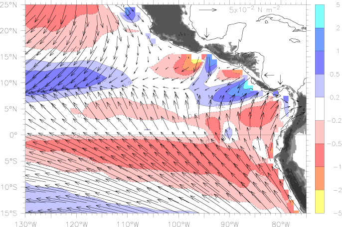
Fig. 1. Mean wind stress (vectors) and wind stress curl (colors) averaged over August 1999–July 2002. Blue shading shows positive curl (upwelling in the northern hemisphere) and red negative curl, in units of 10![]() Nm
Nm![]() , with (stretched) color key at right. The scale vector is in the Gulf of Mexico. Gray shading on land indicates altitudes greater than 250 m. The three mountain gaps referred to in the text are marked with arrows on the Atlantic side; from north to south these jets are denoted Tehuantepec, Papagayo, and Panama.
, with (stretched) color key at right. The scale vector is in the Gulf of Mexico. Gray shading on land indicates altitudes greater than 250 m. The three mountain gaps referred to in the text are marked with arrows on the Atlantic side; from north to south these jets are denoted Tehuantepec, Papagayo, and Panama.
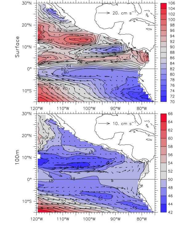
Fig. 2. Mean dynamic height and geostrophic currents relative to 400 m. Top: surface. Bottom: 100 m. Red colors indicate high dynamic heights, blue low (color scales on right). The contour interval is 2 dyn cm. The scale vector for each plot is located in the Gulf of Mexico. Geostrophic current vectors are omitted within ±3° latitude.
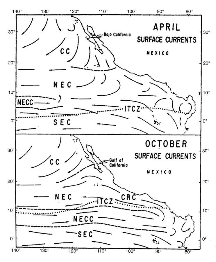
Fig. 3. Annual cycle surface circulation based on ship-drift records (after Baumgartner and Christensen, 1985, which was adapted from Wyrtki, 1965). Current abbreviations are: California Current (CC), North Equatorial Current (NEC), North Equatorial Countercurrent (NECC), South Equatorial Current (SEC) and Costa Rica Coastal Current (CRC). The Intertropical Convergence Zone (ITCZ) is marked by a dotted line. Dashed lines around the NECC show its varying extent.
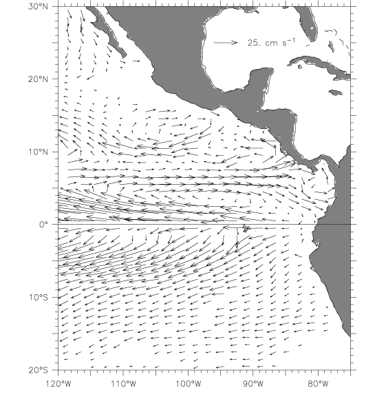
Fig. 4. Mean surface circulation from surface drifters. Vectors were left blank if either the total count of samples in that 1° × 1° box was less than 10, or if fewer than 4 months of the year were represented. The scale vector is located in the Gulf of Mexico.
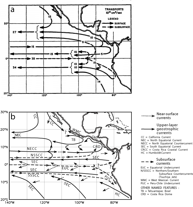
Fig. 5. Schematic three-dimensional circulation in the eastern tropical Pacific. (a) After Wyrtki (1966). (b) The circulation based on modern data. The legend at the right lists the names of currents and features referred to in the text. Several question marks indicate regions where the interconnections among the currents remain unknown (see text).
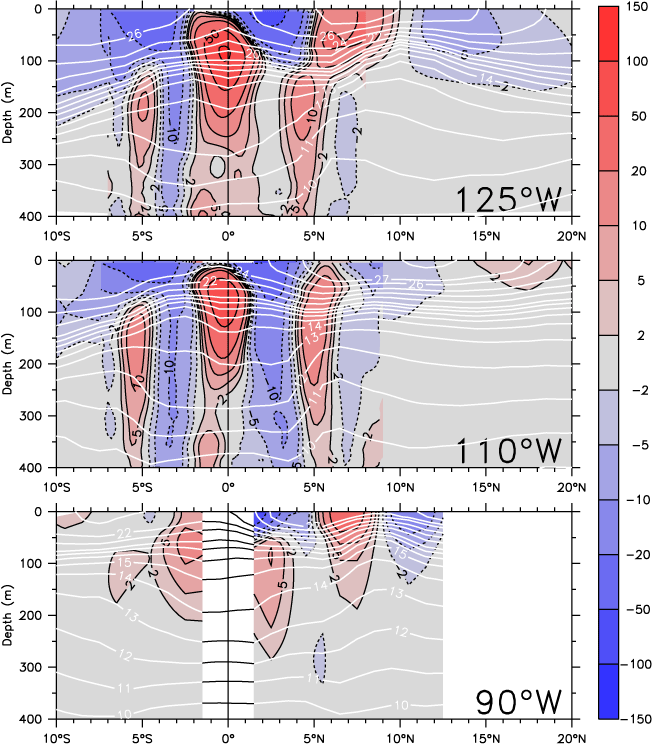
Fig. 6. Mean meridional sections of temperature (white contours) and zonal current (color shading, where red is eastward and blue westward; cm s![]() ) at the three longitudes listed in the lower right corner of each panel. At 125°W and 110°W, directly measured currents are shown within ±8° latitude (see Appendix C.1); elsewhere the currents are geostrophic.
) at the three longitudes listed in the lower right corner of each panel. At 125°W and 110°W, directly measured currents are shown within ±8° latitude (see Appendix C.1); elsewhere the currents are geostrophic.
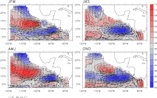
Fig. 7. Annual cycle of surface dynamic height and geostrophic current (relative to 450 m), shown as four average seasons. Red colors indicate high dynamic heights, blue low. The contour interval is 2 dyn cm. The scale vector for geostrophic currents is at lower left. The dynamic height contours shown here have very nearly the same patterns as contours of 20 °C depth for the corresponding season.

Fig. 8. Zonal sections of temperature (top) and meridional geostrophic current (bottom) along 8.5°N, from the coast (right edge) to 110°W. The contour interval for temperature is 1 °C from 8 to 14 °C, then 2 °C from 16 to 26 °C, then 1 °C from 27 to 29 °C; the 20 °C contour is darkened. In the bottom panel, northward current is indicated by solid contours, southward by dashed contours; the contour interval is every 5 cm within ±15 cm s![]() , with additional contours at ±1 and 2, ±0.5 and ±0.2 cm s
, with additional contours at ±1 and 2, ±0.5 and ±0.2 cm s![]() .
.
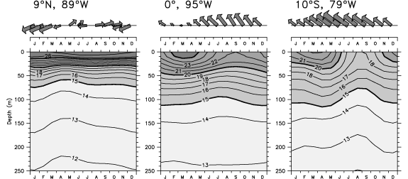
Fig. 9. Average annual cycle of wind stress vectors (top panels) and temperature (bottom panels) at the center of the Costa Rica Dome (9°N, 89°W; left), the equatorial cold tongue (0°W, 95°W; middle) and the Peru coastal upwelling (10°S, 79°W; right). Winds are the ERS scatterometer winds over 1991–2000, and both the length and thickness of the vectors increases with magnitude; the largest vector (June at the coast of Peru) has a magnitude of 5.8 N m![]() . Temperatures are from the AOML XBT data set.
. Temperatures are from the AOML XBT data set.
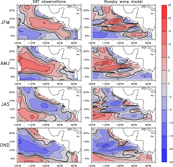
Fig. 10. Comparison of annual cycle anomalies of observed 20 °C depth (left panels) and the Rossby wave model solution (Section 4.2.1) (right panels), for four average seasons (indicated to the left of each row). The common color key is at right, with contour interval of 5 m. Positive values (red) indicate deep anomalies and negative values (blue) indicate shallow anomalies.
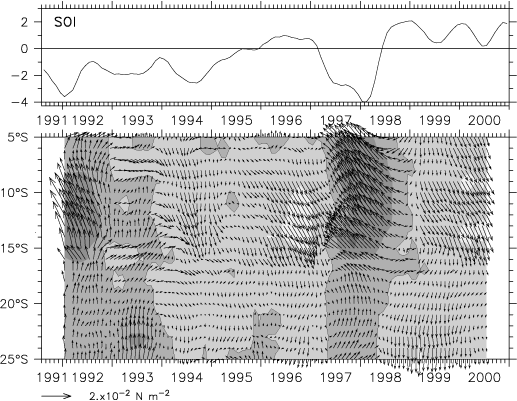
Fig. 11. The Southern Oscillation Index (top) and interannual wind stress anomalies along the coast of Peru (bottom). Interannual anomalies are defined as the 11-month running mean of anomalies from the average annual cycle. Shading shows stress anomaly magnitude, with shading levels every 0.1 N m![]() ; lighter shades show weaker than normal winds, with a contour drawn at zero. The scale vector is at lower left. Negative SOI corresponds to El Nino conditions.
; lighter shades show weaker than normal winds, with a contour drawn at zero. The scale vector is at lower left. Negative SOI corresponds to El Nino conditions.
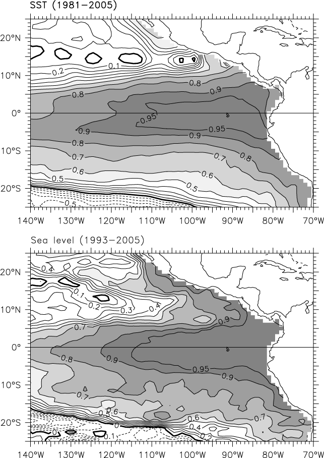
Fig. 12. Correlations of interannually smoothed quantities with the same quantity at 0°W, 95°W. Top: SST from the Reynolds SST product (1981–2005). Bottom: sea level from the Topex/Jason altimeter (1993–2005). Interannual anomalies are defined as the 11-month running mean of anomalies from the average annual cycle. Shading indicates correlations significant at the 95% level (see text).
Return to previous section or return to Abstract