Figure 1. Time series of the SOI (line), OLR intraseasonal rms, averaged in the region 2°S-2°N, 155°E-175°E (dash, W m-2), and zonal wind intraseasonal rms at the TAO mooring at 0°, 165°E (dotted line, m s-1). The SOI is inverted (so El Niño events are positive on the plot).
Figure 2. The structure of the idealized MJO zonal wind stress anomalies along the equator during model year four. Line contours show eastward winds, dashed contours westward winds, with contours at ±1, 2 and 3 × 10⁻² N m-2. The arrows are simply a visual aid to show the direction of each phase of the wind. The winds are described by Eqs. (1)-(3), and represent eastward-advancing oscillations. East of the anomaly region, the forcing remained climatological.
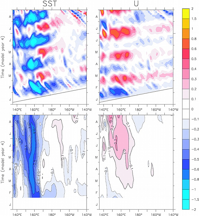
Figure 3. SST and surface zonal current differences along the equator due to oscillating MJO winds. In each case the fields plotted are the difference, during model year 4, between the run with added MJO winds and the control run with climatological winds. (left) SST; (right) zonal current. (top) unsmoothed; (bottom) 60-day running means. The scale for all fields is at right (°C for SST; m s 1 for zonal current). The overlaid slant lines in the top panels show the 1st baroclinic mode Kelvin wave speed for the model stratification (3 m s-1).
Figure 4. Mean surface current difference due to MJOs: the difference between the MJO and the climatological control runs, averaged over four MJO cycles.
Figure 5. Zonal wind stress, wind speed, and latent heat flux at the equator, 150°-170°E, comparing the climatological control run (solid line) and the MJO run (dashed line). (top) zonal wind stress (10-2 N m-2); (middle) wind speed (m s-1) [the dotted line at 4 m s-1 shows the value of the model's gust factor, see section 3b(1)]; (bottom) Latent heat flux (W m-2, with negative values indicating heat loss by the ocean).
Figure 6. Mean heat flux difference terms (the difference between the MJO and the climatological control runs) averaged over four MJO cycles (W m-2). (top) Latent heat flux; (middle) zonal advection heat flux; (bottom) vertical advection heat flux. Negative values (cooling the ocean) are shaded; positive values are hatched.
Figure 7. SST (shading and contours) and zonal winds (vectors) on the equator during the coupled model runs. (top) control run hindcast initialized to 1 Jan 1997. (bottom) Difference between the control run and the run with the OGCM SST imposed. Note the different contour intervals in each panel.
Return to previous section or go to Abstract