| Source | df | Mean square | F | p |
|---|---|---|---|---|
| Strata | 9 | 2.7509 | 3.89 | 0.0003 |
| Day/night | 1 | 0.2462 | 0.35 | 0.5562 |
| Interaction | 9 | 0.8936 | 1.26 | 0.2639 |
| Error | 112 | 0.7064 | ||
U.S. Dept. of Commerce / NOAA / OAR / PMEL / Publications
Catch rates of walleye pollock larvae did not vary significantly between day and night (ANOVA, p = 0.56, Table 1). There was no consistent pattern of catch in the day or the night. The strata effect was highly significant (ANOVA, p = 0.0003, Table 1).
| Source | df | Mean square | F | p |
|---|---|---|---|---|
| Strata | 9 | 2.7509 | 3.89 | 0.0003 |
| Day/night | 1 | 0.2462 | 0.35 | 0.5562 |
| Interaction | 9 | 0.8936 | 1.26 | 0.2639 |
| Error | 112 | 0.7064 | ||
The catch rates of the bongo and the 1 m Tucker trawl did not differ significantly (K-S test, p = 0.89). Other work on catchability of larvae by these gear types (Shima & Bailey unpubl. data) has also shown no consistent pattern of differing efficiency over this larval size range. The gear comparison experiments showed that the 1 m Tucker trawl was effective in catching the entire length-range of larvae that were caught by the other gear (Fig. 2). The 3 m Tucker trawl and the Methot trawl caught less than the bongo and the 1 m Tucker because of their large mesh sizes. There were not significant numbers of smaller larvae in the 0.333 mm mesh bongo, or larger larvae in the larger mesh 3 m Tucker or Methot trawls. Therefore, no correction of abundance estimates for escapement or avoidance was made to the survey station catches made with the 1 m Tucker trawl.
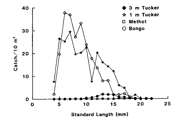
Fig. 2. Theragra chalcogramma. Comparison of catch at length of walleye pollock larvae averaged over all hauls from the 4 gear types.
Estimates of probable changes in larval distribution derived from the application of the advection and diffusion model resulted in dropping the 2 northernmost stations from the Pass 2 survey. Larvae found at these 2 stations would have been upstream of the survey area in Pass 1 and therefore would have been advected into the Pass 2 survey area. Otherwise, the boundaries for Pass 2 were not changed, as the model predicted that more than 95% of the larvae found in Pass 1 would be found within the area covered during Pass 2.
Comparison of the larval concentrations predicted from the model and those
observed on the second survey (Fig. 3) shows
that patch structure observed in the field was not preserved due to diffusion
in the model, for all reasonable values of diffusivity (K > 5 � 10
 cm
cm s
s ).
).
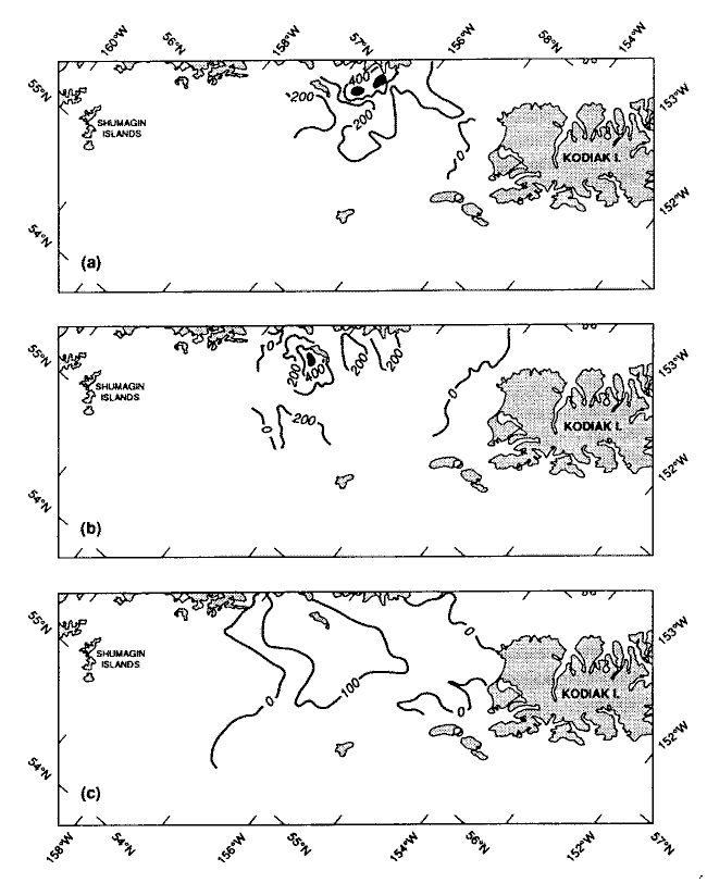
Fig. 3. The domain of the model is shown. Distribution of larvae (a) found
during Pass 1 (this is the initial condition for the model), (b) found during
Pass 2, and (c) predicted by the model of advection and diffusion for the time
period corresponding to Pass 2. Larval abundance contours shown are in. 10 m (solid area: >600 larvae 10 m).
Abundances of the 10 April through 16 May cohorts were used to estimate mortality rates. Abundances for the 10 through 28 April cohorts were very similar between Passes 1 & 2. Abundances of fish with hatch dates between 1 and 16 May showed a clear decline in abundance from the first to the second pass (Fig. 4).
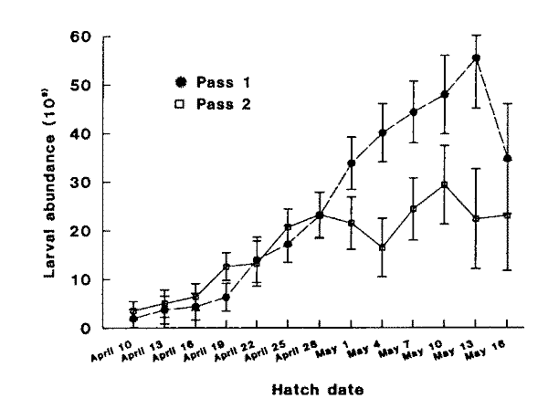
Fig. 4. Theragra chalcogramma. Larval abundance for 3 d cohorts during Passes 1 and 2.
The instantaneous daily mortality rates (z) for the separate 3 d cohorts
ranged from –0.0574 to 0.0757 d (Table
2). The instantaneous daily mortality rate for the combined 10 April to 16 May
cohorts was z = 0.033 d (Var(z)
= 0.0013). This mortality rate was not significantly different from zero (t
= 0.92, p > 0.20).
| Hatch | Age (d) | Abundance of larvae in survey area | z (d)
|
SE | ||||
|---|---|---|---|---|---|---|---|---|
| date | Pass 1 | Pass 2 | Pass 1 | Pass 2 | ||||
| Numbers | SE | Numbers | SE | |||||
| 10 Apr | 42 | 54 | 1.971 � 10 |
1.891 � 10 |
3.564 � 10 |
2.569 � 10 |
-0.0494 | 0.1000 |
| 13 Apr | 39 | 51 | 3.718 � 10 |
2.845 � 10 |
5.043 � 10 |
3.486 � 10 |
-0.0254 | 0.0859 |
| 16 Apr | 36 | 48 | 4.381 � 10 |
2.749 � 10 |
6.365 � 10 |
3.191 � 10 |
-0.0311 | 0.0669 |
| 19 Apr | 33 | 45 | 6.336 � 10 |
2.845 � 10 |
1.261 � 10 |
4.875 � 10 |
-0.0574 | 0.0494 |
| 22 Apr | 30 | 42 | 1.400 � 10 |
4.656 � 10 |
1.322 � 10 |
4.128 � 10 |
0.0048 | 0.0380 |
| 25 Apr | 27 | 39 | 1.721 � 10 |
3.752 � 10 |
2.070 � 10 |
5.480 � 10 |
-0.0154 | 0.0286 |
| 28 Apr | 24 | 36 | 2.308 � 10 |
4.712 � 10 |
2.323 � 10 |
5.631 � 10 |
-0.0005 | 0.0264 |
| 1 May | 21 | 33 | 3.384 � 10 |
5.401 � 10 |
2.151 � 10 |
5.205 � 10 |
0.0377 | 0.0242 |
| 4 May | 18 | 30 | 4.008 � 10 |
5.991 � 10 |
1.646 � 10 |
4.018 � 10 |
0.0742 | 0.0239** |
| 7 May | 15 | 27 | 4.430 � 10 |
6.377 � 10 |
2.435 � 10 |
5.016 � 10 |
0.0499 | 0.0209** |
| 10 May | 12 | 24 | 4.788 � 10 |
8.078 � 10 |
2.930 � 10 |
6.166 � 10 |
0.0409 | 0.0225* |
| 13 May | 9 | 21 | 5.536 � 10 |
1.027 � 10 |
2.233 � 10 |
5.590 � 10 |
0.0757 | 0.0260** |
| 16 May | 6 | 18 | 3.466 � 10 |
1.130 � 10 |
2.296 � 10 |
6.020 � 10 |
0.0343 | 0.0349 |
* Significantly different from zero ( = 0.05)
 |
||||||||
| ** Significantly different from zero (
= 0.01) |
||||||||
Inspection of the cohort distributions for Pass 1 (Fig. 5) showed an area of relatively high concentration of larvae from the 10 to 19 April cohorts on the northwest side of the survey area near the Alaska Peninsula, which might not have been fully sampled. This was of interest due to the fact that the mortality rates estimated for these 4 cohorts were negative (Table 2). To test whether a significant number of larvae might have been missed in the inshore area during Pass 1 (which would have lowered the mortality rates for these cohorts), the northwest boundary of the survey area was redrawn closer to the Alaska Peninsula, increasing the total survey area for Pass 1. Larval abundances were extrapolated to the new boundary, and mortality rates recalculated using new total cohort abundances for Pass 1. The results of this analysis showed that, unless unusually high abundances of larvae were present in the nearshore areas outside the Pass 1 grid, extension of the survey area would not have been sufficient to raise the estimates of the mortality rates for these cohorts above zero (Table 3).
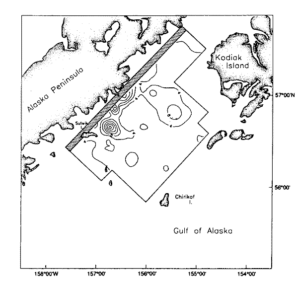
Fig. 5. Theragra chalcogramma. Distribution of the 19 April cohort
during Pass 1 showing area on the northwest border of the survey area (shaded
where larvae might have been missed, causing underestimation of mortality rates.
Larval abundance contours shown are ind. 10 m.
| Hatch date | Mortality rate | Mortality rate | % Change in |
|---|---|---|---|
(uncorrected) |
(corrected) |
mortality rates | |
| 10 Apr | -0.0494 | -0.0432 | +12.5 % |
| 13 Apr | -0.0254 | -0.0174 | +31.5 % |
| 16 Apr | -0.0311 | -0.0217 | +30.2 % |
| 19 Apr | -0.0574 | -0.0462 | +19.7 % |
| Using original Pass 1
survey boundary |
|||
| Using extended Pass 1
survey boundary |
|||
The overall daily mortality rate for each pass derived from the catch curve
analysis was z = 0.0838 d for Pass
1, and z = 0.0421 d for Pass 2.
Three main areas of concentration of larvae are visible in the distribution of the combined 10 April to 16 May cohorts in Pass 1 (Fig. 6a). Two patches were found to the northeast of Sutwik Island near the Alaska Peninsula ("Patch 1" and "Patch 2"), and one was found to the northeast of the Semidi Islands ("Patch 3"). Three concentrations of larvae also are visible in Pass 2 (Fig. 6b), one to the northeast of Sutwik Island ("Patch 1"), one to the southwest of Sutwik Island ("Patch 2"), and one to the south of the Semidi Islands ("Patch 3"). Most of the 3 d cohorts were present in all 3 of these main patches in each pass.
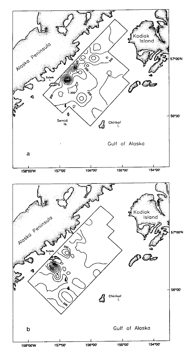
Fig. 6. Theragra chalcogramma. Distribution of 10 April to 1 May
cohorts during (a) Pass 1 and (b) Pass 2. Larval abundance contours shown are
ind. 10 m.
There was an apparent southwestward displacement of all 3 patches over the interval between passes. By assuming the coherence of these 3 patches and measuring their displacement between the 2 passes, we could use their net movement over this time period as an estimate of the rate of larval drift. The time period over which movement was estimated was between the actual sampling dates at each patch rather than between the mean pass dates. Drift was calculated from the straight-line movement of patches between the 2 dates.
Patch 1 movement averaged 2.59 cm s, Patch
2 averaged 3.61 cm s, and Patch 3 averaged
5.29 cm s. The average rate of drift for
all 3 patches was 3.8 cm s.
Rates of drift were also estimated from displacement of the centroids of the
entire larval distributions for each pass. The location of the centroids for
1988 in Passes 1 & 2 were similar to 1981 and 1986 (Fig.
7). The centroid locations for 1979 and 1982 were further offshore. Centroid
locations appear farther offshore than might be indicated by the distributions
shown in the contour plots because the few high stations represented in the
patches do not have a large impact on centroid locations, whereas they are interpolated
over a larger area in the contour plots. The displacement of the centroids over
the 12 d between mean pass dates suggests a rate of drift of 3.9 cm s.
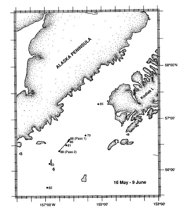
Fig. 7. Theragra chalcogramma. Centroids of larval distributions in Passes 1 and 2 (May 1988), as compared with other years (figure adapted from Kendall and Picquelle 1990).
The net movement of the satellite-tracked buoy was compared to these 2 estimates
of larval drift. The buoy was deployed on 24 May, near the center of Patch 1
(which was sampled at approximately this time) (Fig.
8). The buoy location on 31 May was close to the center of Patch 1 when
it was sampled during Pass 2 (on 1 June). If only the period 24 May to 1 June
was considered (corresponding approximately to the interval between the passes),
the average velocity was 4.7 cm s.
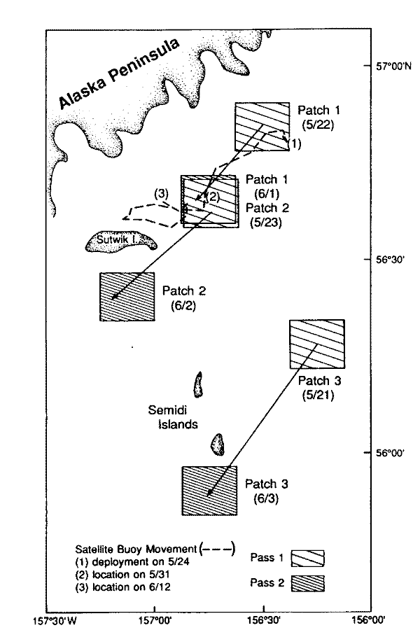
Fig. 8. Theragra chalcogramma. Boxes show the locations of the 3 main concentrations of larvae (as seen in Fig. 6a, b) and their net displacement between passes. The track of the satellite-tracked buoy is also shown.
Return to previous section or go to next section