 heating in the upper 250 m averaged over the region 152°W to 110°W.
U.S. Dept. of Commerce / NOAA / OAR / PMEL / Publications
Time series of surface wind and upper ocean temperature and velocity, obtained from equatorial moorings along 110°W, are used to assess the importance of various oceanic and atmospheric processes in the variation of the mixed layer temperature for the period January 1986 to June 1988. This period coincides with the onset and development of the 1986-87 El Nińo-Southern Oscillation warm event and a subsequent cold event in 1988. Results of the temperature equation analyses indicate that seasonal and interannual variability of sea surface temperature (SST) in the eastern Pacific cannot be accounted for by observed surface heat flux; oceanic processes play an important role in the heating of the surface water. Although no single process dominated SST change, the most important processes in the mean balance were the net incoming surface heat flux, the penetrative solar radiation, and the vertical turbulent flux out the bottom of the mixed layer. The mean vertical entrainment could not be estimated with the available data. On the seasonal time scales, both the vertical turbulent heat flux and the vertical entrainment variations were well correlated with SST change. Zonal advection was a significant contribution to the heat flux variability, but its fluctuations were poorly correlated with the mixed layer heating. In particular, it was found that zonal advective heat flux tended to be out of phase with the spring warming. At higher frequencies, little zonal advective heat was found to be associated with the passage of a Kelvin event in January 1987. Surprisingly, meridional heat advection appeared more important than the zonal heat advection in modifying the local SST as this event passed the mooring location.
Improved understanding of the El Nińo-Southern Oscillation (ENSO) phenomena in the Pacific Ocean has received increased attention in recent years as the importance of these signals in the year-to-year variations of the global climate has become apparent [Philander, 1990]. Crucial to this understanding is an accurate description of the processes which maintain and change the tropical Pacific sea surface temperature (SST) and the interaction of these oceanic changes with the atmosphere. The important processes are likely to vary with location and at least three regimes in the equatorial Pacific can be identified based on atmospheric and oceanic conditions. In the western Pacific the surface warm layer is thick (although salinity may provide an important source of shallow stratification), SST is high and changes little seasonally, and the mean winds are weak but their variability is large. In the central Pacific, SST has a weak seasonal signal but relatively large interannual changes which are climatically significant; the southeast trade winds are generally strong except during ENSO events. In the eastern Pacific the thermocline is very shallow, near-equatorial waters are relatively cool, and SST gradients are large. The prevailing winds have a strong cross-equatorial component and both the winds and the SST vary annually.
Several recent studies address the upper ocean heat budget and SST changes
near the equator. Wyrtki
[1981] used climatological data to estimate the mean heat budget for a 50-m-deep
box from 170°E to 100°W, 5°N to 5°S. Meridional and vertical diffusion was negligible
in his calculation. The net surface heating was balanced by zonal and meridional
advection which included the contribution from upwelling. Enfield
[1986] expanded this study to include the entire equatorial band and to
examine seasonal variations. Based on Enfield's "best guess" mean
heat budget, all of the possible terms in the upper ocean heating appear to
be significant. In the western Pacific the balance was primarily between surface
heat gain and vertical diffusion. In the central Pacific, atmospheric fluxes
and meridional diffusion contribute nearly equal warming; this heat is removed
by zonal and meridional advection (which includes upwelling) and by vertical
diffusion. In the eastern Pacific near 110°W, the surface heating (about 30%
of which is due to meridional diffusion) is primarily offset by meridional advection
and vertical diffusion. Bryden
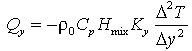
and Brady [1989] emphasized the importance of the meridional eddy diffusion
which in their calculation contributed 245 W m
heating in the upper 250 m averaged over the region 152°W to 110°W.
In the western Pacific, Meyers et al. [1986] pointed out the importance of variations in latent heat flux in cooling the warm pool during the 1982-83 ENSO episode. Similarly, McPhaden and Hayes [1991] found that evaporative cooling was important in the day-to-month SST changes and also noted the role of zonal advection. Stevenson and Niiler [1983] examined the heat budget in the central Pacific and concluded that on seasonal time scales, the surface heat flux was a major factor determining the evolution of SST. Zonal advection was not found to be as important. In the eastern Pacific zonal advection appears to be an important contribution to the warming during ENSO [Halpern et al., 1983; Mangum et al., 1986; Philander and Hurlin, 1988; McPhaden and Hayes, 1990].
In this paper we present the results of a study of the surface mixed layer heat budget estimated from moored array data along 110°W during 1986-88. The analysis focuses on the seasonal and lower frequency variability. This period encompasses an ENSO cycle and includes the onset and development of the 1986-87 warm event and the onset of the subsequent cool event. The near equatorial variability at 110°W during these years and its relation to the evolution of conditions throughout the equatorial Pacific are described in McPhaden and Hayes [1990] (hereinafter referred to as MH). Briefly, MH noted the onset of warm SST anomalies at 0°, 110°W in mid-1986; an increase in these anomalies and a concomitant decrease in the strength of the South Equatorial Current (SEC) in September-November 1986; and persistence of the warm SST throughout 1987. In early 1988 the SST rebounded rapidly, and cold anomalies in excess of 3°C appeared in association with a large scale shoaling of the thermocline. Much of the year-to-year variability at 110°W appeared to result from zonal wind variations in the central and western Pacific.
In the present study, the moored array data used in MH are combined with other nearby measurements and climatology to describe the mixed layer variability on seasonal and interannual time scales and to estimate terms in the heat budget. The purpose is to attempt to quantitatively compare the relative importance of various physical processes in the evolution of the SST in the eastern Pacific. This region is of particular interest in simplified coupled models of ENSO [Cane and Zebiak, 1985; Battisti, 1988]. The shallow thermocline contributes to large SST changes associated with local and remote wind stress variations and these SST fluctuations can in turn yield changes in the local surface wind [Wallace et al., 1989; Hayes et al., 1989b]. Understanding the mechanisms of SST change in the eastern Pacific is fundamental in order to accurately model the coupled ENSO phenomena.
The measurements used in this study consist of wind, temperature, and current data from the locations and during the periods detailed in Figure 1. Data gaps of less than 2 weeks were filled by linear interpolation. Off the equator, only data during December to May of each year were used, and gaps in SST were filled using the data at 20-m depth. The equatorial instrumentation and processing procedures are discussed in MH. Off-equatorial measurements were collected by ATLAS wind and thermistor chain moorings. ATLAS is a taut wire surface mooring which measures wind (at 4 m above sea level), air temperature, SST (at 1 m depth), and 10 subsurface temperatures to a maximum depth of 500 m. All data are telemetered in real time via Service Argos. In the data sets used here the transmitted temperature data were all 24-hour averages; the wind averaging interval varied. However, in subsequent processing, all time series were reduced to daily averages. The ATLAS mooring and thermistor chain is discussed further by Milburn and McLain [1986] and Hayes et al. [1989a, 1991].
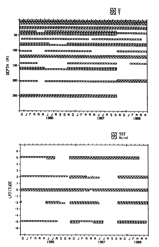
Fig. 1. Depths and locations of the time series used in this study. (Top) Record lengths of the velocity (u) and temperature (T) time series at 0°, 110°W. (Bottom) SST and wind record lengths at the measurement locations along 110°W. SST was measured at 1 m depth except at 5°S for January-August 1986, when the 20 m temperature record was used.
Time series of the equatorial data are shown in Figure 2. The monthly average climatology shown in this figure was computed from the mooring time series as described in MH. Warmest SST (28.5°C) occurred in April 1987; the largest positive anomaly was in September 1987 (3.4°C). Throughout the period September 1986 to February 1988, SST was above normal. Then from March to May 1988, SST dropped by nearly 8°C; the ENSO warm event had ended and a cold event began. This shift from warm to cold was much more dramatic than the onset of the warm period.
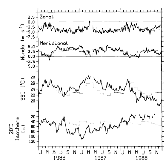
Fig. 2. Time series of zonal and meridional surface wind, SST, and depth of the 20°C isotherm at 0°, 110°W for the 3 years 1986-1988. Solid lines are the measured values, and dotted lines are the monthly mean climatological values based on the historical data from the mooring at this location [McPhaden and Hayes, 1990].
Surface wind tended to follow the annual cycle throughout the study period. Meridional winds were anomalously strong the last half of 1986 and through 1987. Zonal winds were also stronger than normal in much of 1987. The onset of cooler than normal conditions in 1988 was accompanied by normal zonal and weaker than normal meridional winds. MH note that this pattern of surface wind is consistent with the analysis of climatological data [Wallace et al., 1989] which shows that near the equator the southeast trades in the eastern Pacific are stronger than normal during ENSO warm events. Wallace et al. [1989] attribute this result to reduced atmospheric boundary layer stratification and shear when SST exceeds surface air temperature.
Thermocline depth as represented by the 20°C isotherm in Figure 2 tends to mirror SST on interannual time scales. The thermocline was anomalously deep for about 1 year beginning in September 1987, when SST was anomalously warm. The shallowest thermocline was in 1988 when SST was anomalously cool. However, higher-frequency correlations between SST and 20°C depth are not so apparent. There are several examples of large-amplitude changes in 20°C depth which are not seen in SST (e.g., the January 1987 deepening), and the seasonal cycle in SST was not observed in thermocline depth.
Seasonal and lower-frequency variability was examined by low-pass filtering the time series with a 91-day Hanning filter. This filter has a zero at 45 days and passes 50% of the variance at 91 days. On seasonal time scales the correlations among SST, surface wind speed, and total surface heat flux from the atmosphere to the ocean (estimated as discussed in section 3) are apparent in Figure 3 where the time series with the mean value removed are plotted. SST and surface wind speed tend to be out of phase. Net surface heat flux tends to mirror the surface wind speed. Hence warmest SST and largest surface heat flux occur nearly simultaneously each year. This result implies that oceanic processes must be important in the heat budget of the surface waters in the eastern equatorial Pacific. Otherwise, surface heat flux and SST change (rather than SST) would be in phase. The oceanic processes and their estimation from the moored array data are discussed in the next section.
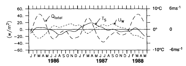
Fig. 3. Low-pass-filtered (91-day Hanning filter) time series of the SST (T , solid line), surface wind speed (U
 , short-dashed line), and total surface heat flux
(Q
, short-dashed line), and total surface heat flux
(Q , long-dashed line, see text) at
0°, 110°W for the period indicated. The mean value has been removed from each series
prior to plotting. Scales for Q are
on the left-hand axis; T and U are indicated on the right.
, long-dashed line, see text) at
0°, 110°W for the period indicated. The mean value has been removed from each series
prior to plotting. Scales for Q are
on the left-hand axis; T and U are indicated on the right.
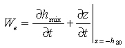
To investigate the processes which lead to the SST changes shown in Figures
2 and 3, we examined the heat budget of the
surface mixed layer using the formalism discussed in McPhaden
[1982]. With the assumption of vertically uniform mixed layer temperature
of depth h , the mixed layer
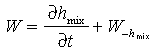
temperature equation can be written as:
, the mixed layer
temperature equation can be written as:
![]() (1)
(1)
with
![]()
![]()
The rate of change of sea surface temperature, T,
is expressed in terms of Q .
The density of seawater is
.
The density of seawater is 
 = 1022.4 kg m
 and the heat capacity is C
 = 3.94 × 10
 J kg
J kg °C. The net surface heat flux from the atmosphere
into the mixed layer ( Q
°C. The net surface heat flux from the atmosphere
into the mixed layer ( Q )
is composed of the shortwave (Q
)
is composed of the shortwave (Q ),
longwave (Q
),
longwave (Q ), latent (Q
 ),
and sensible (Q
),
and sensible (Q ) heat fluxes
and the penetrative radiation (Q
) heat fluxes
and the penetrative radiation (Q )
at the bottom of the mixed layer. The oceanic processes (Q
)
at the bottom of the mixed layer. The oceanic processes (Q )
which contribute to changes in mixed layer temperature are zonal (Q
)
which contribute to changes in mixed layer temperature are zonal (Q )
and meridional (Q
)
and meridional (Q ) advection,
entrainment cooling across the base of the mixed layer ( Q),
and vertical (Q
) advection,
entrainment cooling across the base of the mixed layer ( Q),
and vertical (Q ) and meridional
(Q
) and meridional
(Q ) eddy heat flux. Zonal
eddy heat flux has been ignored, since previous studies suggest that it is small
[Bryden
and Brady, 1985].
) eddy heat flux. Zonal
eddy heat flux has been ignored, since previous studies suggest that it is small
[Bryden
and Brady, 1985].
The terms in the surface heat flux into the mixed layer can be estimated using the bulk formulae. These relations are discussed in several recent references [e.g., McPhaden, 1982; Stevenson and Niiler, 1983; Reed, 1983; Dobson and Smith, 1988; Weare, 1989]. The equations used here are those of Reed [1983]; their accuracy is evaluated in Dobson and Smith [1988]. Specifically, the surface heat flux terms in (1) are given by:
![]() (2)
(2)
![]() (3)
(3)
![]() (4)
(4)
![]() (5)
(5)
![]() (6)
(6)
In (2), Q is the clear sky radiance [Reed,
1977, 1983],
C the cloudiness (tenths) and
is the clear sky radiance [Reed,
1977, 1983],
C the cloudiness (tenths) and  is the
noon solar altitude (degree). The clear sky radiance and alpha are evaluated
using a harmonic formula which introduces latitudinal and annual variations.
In (3),
is the
noon solar altitude (degree). The clear sky radiance and alpha are evaluated
using a harmonic formula which introduces latitudinal and annual variations.
In (3),  =
0.97 is the emissivity of the ocean;
=
0.97 is the emissivity of the ocean; ![]() = 5.67 × 10
= 5.67 × 10 W m
°K
W m
°K is the Stefan-Boltzmann constant, e
is the atmospheric vapor pressure. In (4) and
(5),
is the Stefan-Boltzmann constant, e
is the atmospheric vapor pressure. In (4) and
(5),  = 1.15 × 10g cm
is the air density, C
= 1.15 × 10g cm
is the air density, C = 1.2
× 10 is the exchange coefficient, L
= 2440 J g is the latent heat of vaporization,
V is the wind speed at a nominal height of 10 m, q
is the specific humidity saturated at the sea temperature, q
is the specific humidity of the air at 10 m elevation, and T
and T are the air and sea
temperatures. Equation (6) estimates the heat
loss by radiation which penetrates through the mixed layer. This exponential
decay law is taken from Ivanov
[1977] with
= 1.2
× 10 is the exchange coefficient, L
= 2440 J g is the latent heat of vaporization,
V is the wind speed at a nominal height of 10 m, q
is the specific humidity saturated at the sea temperature, q
is the specific humidity of the air at 10 m elevation, and T
and T are the air and sea
temperatures. Equation (6) estimates the heat
loss by radiation which penetrates through the mixed layer. This exponential
decay law is taken from Ivanov
[1977] with ![]() =
0.04 m. The mixed layer depth, h,
is estimated as discussed below.
=
0.04 m. The mixed layer depth, h,
is estimated as discussed below.
The mooring measurements provided information on wind speed, SST and air temperature.
In order to apply equations (2-5), we used the mooring data supplemented by
Comprehensive Ocean-Atmosphere Data Set (COADS) marine surface climatology.
Measured winds and air temperature were used without correcting the measurement
height to 10 m. Assuming a logarithmic profile with neutral stability and a
constant drag coefficient of 1.2 × 10 [Large
and Pond, 1982], an increase of wind speed by 8% would account for the
measurement height. This correction was not made because of the uncertainties
in the assumptions used to derive it. The saturation humidity q
in (4) was evaluated from the Clausius-Clapeyron
equation using the observed SST. Cloud cover and relative humidity were obtained
from a monthly mean COADS climatology for 1946-85 [Deser,
1989]. For comparison, monthly mean values based on COADS data for 1986-1988
were also used (C. Deser, personal communication, 1989). Liu
and Niiler [1990] discuss the sensitivity of the latent heat flux to
variations in humidity.
After smoothing with a 91-day Hanning filter, the estimated surface flux terms
are shown in Figure 4. The incoming shortwave
radiation is based solely on climatology. It has a semiannual variation associated
with the sun passing over the equator twice each year. No interannual variability
is possible because climatological monthly cloud cover is used in (2).
The mean value is about 250 W m and the
standard deviation of the low pass filtered time series is about 15 W m.
These results are consistent with Reed
[1983].
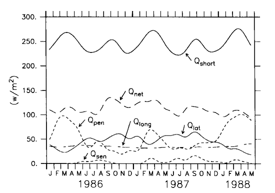
Fig. 4. Components of the surface heat flux (see equation (1)).
The estimated latent heat flux undergoes both annual and interannual variations. Latent
heat flux is minimum in March, when wind speed is low (Figure 3),
and maximum in boreal autumn. The minimum in March of 1987 is almost twice the March value
in 1986 or 1988. This increase in latent heat release is related to the warm SST anomalies
and higher wind speeds that occurred in the eastern Pacific during the 1987 El Nińo. The
mean latent heat flux is approximately 45 W m , which
again agrees with Reed's result, and the standard deviation is about 12 W m.
The longwave radiation is almost a constant value of 35 W m
over the record length and thus does not contribute significantly to the change
in the total heat flux. The sensible heat flux depends on the air-sea temperature
difference. Previous studies in the Pacific Ocean [Reed,
1977, 1983;
Weare
et al., 1981; Esbensen
and Kushnir, 1981] have shown that this heat flux is small (about 10
W m). Since some of the air temperature
data are missing from the equatorial mooring record, we were unable to compute
the sensible heat flux over the entire record length. However, whenever possible
the calculation was made and the mean (and standard deviation) of Q
was less than 5 W m. Thus Q
was ignored in subsequent calculations.
Because mixed layer depth is shallow in the eastern Pacific, incoming solar
radiation cannot be completely absorbed within the layer. On average, about
50 W m penetrates into the deep ocean. This
penetrative radiation is strongest during springtime when the mixed layer is
shallow (Figure 5). Thus although the solar radiation
is strongest in spring season, the net heating received by the mixed layer is
not necessarily largest at that time. Indeed, the net heating within the mixed
layer, Q, in Figure
4, is maximum in the fall of 1986. The penetration of radiation through
the mixed layer reduces the annual variation of the net solar heating. The mean
value of the net heating within the mixed layer is 115 W m
with a standard deviation of 10 W m. The
mean heat flux at the surface is 165 W m,
comparable to the 150 W m value determined
by Reed
[1983] for the eastern equatorial Pacific.
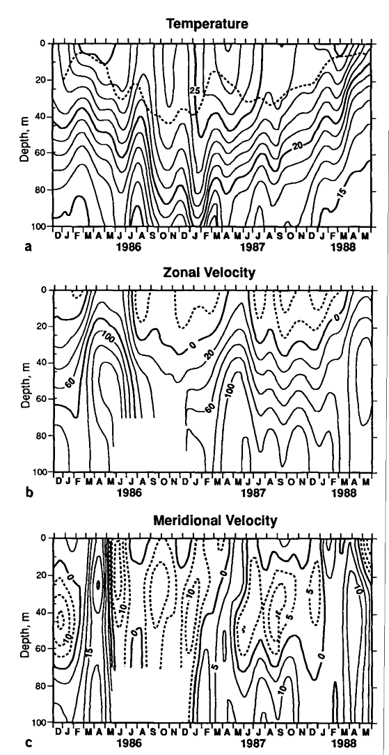
Fig. 5. Contour plots of (a) isotherm depth (contours are in degrees
Celsius), (b) zonal velocity (centimeters per second), and (c) meridional
velocity (centimeters per second) in the upper 100 m at 0°, 110°W, based on the 91-day
low-pass-filtered time series. The dashed line superimposed on the isotherm contours
indicates the mixed layer depth computed as discussed in the text. Contour intervals are
1°C, 20 cm s, and 5 cm s for temperature, zonal velocity, and meridional velocity,
respectively.
Sources of errors in Q
can come from both random and systematic uncertainties in the basic observations
and in the parameters in the bulk formulae. Recent studies by Weare
[1989] indicate that the uncertainties in monthly mean climatological estimates
of the surface heat flux components over the eastern tropical Pacific are 20
W m for the solar radiation, 10 W m
for longwave radiation, 35 W m for latent
heat flux, and 5 W m for sensible heat flux,
which leads to a total error of 40 W m for
the net surface heat flux. The uncertainties of the variability of heat fluxes
should be smaller than the error in absolute flux because systematic errors
in the observations and bulk formulae may cancel upon differencing. However,
our estimates have an additional uncertainty associated with the use of climatological
data combined with mooring data for specific years. Comparison of the fluxes
computed from climatological values of cloud cover and relative humidity (Figure
4) with those estimated using 1986-1988 COADS data show an rms difference
of about 10 W m. Thus, the deviations from
climatology of cloud cover and humidity during the study period were relatively
small. The climatological values were used in the remaining calculations since
the statistical reliability of these estimates is higher.
The moored temperature and velocity measurements on the equator (Figure 1) were interpolated, using a Laplacian interpolation scheme, to an evenly spaced grid from zero to 100 m with a resolution of 5 m. These gridded data were used in all subsequent calculations discussed here, and all derived quantities were low passed filtered with a 91-day Hanning filter prior to further analysis.
Figure 5 shows contour plots of the gridded and filtered
temperature and velocity data. Superimposed on the temperature contours is the time series
of mixed layer depth (h). This h was estimated by finding the depth at which the
contoured temperature was 0.5°C less than the SST. Linear interpolation was used between
grid points. If the mixed layer was less than 5 m, it was set equal to 5 m. Note that the
instrument resolution (Figure 1) restricts the accuracy of
the depth determination to at best about ±5 m. The mixed layer was shallow in boreal
spring and deepest in late summer or fall. On the seasonal time scale mixed layer depth
and SST tend to be out of phase: warmest SST corresponds to a shallow mixed layer.
However, the mixed layer in March 1987, during the ENSO warm event, was deeper than in
either 1986 or 1988. The shallowest mixed layer occurred in spring 1988. Initially, from
January to March 1988, this shoaling was associated with the seasonal warming; however,
the mixed layer continued to be shallow as the SST dropped by nearly 8°C from March to
May 1988. During this period the stratification extended to the surface and our
approximation which assumes an isothermal surface layer is invalid.
The time rate of change of the mixed layer temperature (Q) was estimated from the data in Figure 5 using centered differences in time (Figure 6a, solid curve). The mixed layer heating
assuming a constant layer thickness of 25 m (Figure 6a,
dashed line) is also shown, since the estimate of mixed layer depth may be questionable
given the vertical resolution of the instruments. The effect of the mixed layer depth
variation was most important during January-February 1986 and January-May 1988, when the
mixed layer was very shallow. During these periods, the amplitude of heating fluctuations
computed from the variable mixed layer depth are considerably smaller than those obtained
with a constant depth. In the latter period this difference amounted to nearly 60 W m. The constant mixed layer case indicated the rapid
decrease in SST.
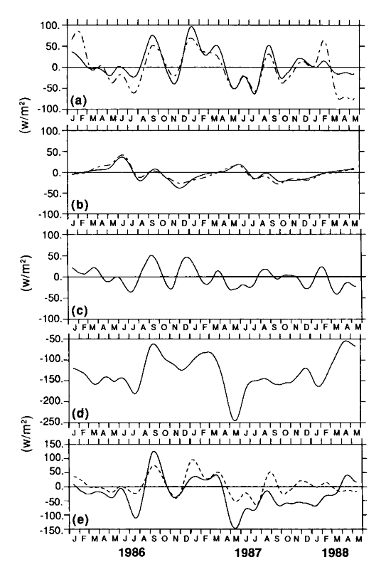
Fig. 6. Time series plots of various terms in equation (1). All time series have
been low pass filtered with a 91-day Hanning filter. ( a) Change in the mixed layer
heat content, Q; the solid line was
computed with variable h, and the
dashed line has a constant h = 25 m.
(b) Zonal advective heat flux, Q ; the solid line was computed with
  T/x estimated from moorings at 110°W and 140°W, dashed
line assumes a constant
T/x estimated from moorings at 110°W and 140°W, dashed
line assumes a constant ![]() . (c) Vertical entrainment, Q. (d) Vertical diffusive heat flux, Q. (e) Superposition of Q (dashed line) and Q
. (c) Vertical entrainment, Q. (d) Vertical diffusive heat flux, Q. (e) Superposition of Q (dashed line) and Q (solid line) as defined in the text.
Over the record length, the mean Q
(using the variable h) was about 6 W
m with a standard deviation of 33 W m. Qualitative comparison of this mixed layer heating and
net solar heat flux (Q, Figure 4) indicates large differences in the mean value and
little correlation of the variability. The mean Q exceeds Q by more than
100 W m and the amplitude of Q fluctuations are too small to balance the
changes in mixed layer heating. Evidently, the variability of mixed layer temperature must
result from low-frequency imbalances of Q and the ocean processes included in equation (1).
The terms in (1) which can be estimated from the long
equatorial time series are discussed below.
Zonal heat advection can be estimated from the moored velocity data at 110°W (Figure 5) and a measure of the zonal temperature gradient, T .
.
![]() (7)
(7)
The vertically averaged zonal velocity of the mixed layer is u. This velocity
was estimated using the gridded, low-pass-filtered time series shown in Figure 5b, using the mixed layer depth shown in Figure 5a. A time series of T was estimated from the moored temperature
measurements at 110°W and 140°W (the 140°W time series are discussed in MH). Since the
local temperature gradient at 110°W may be poorly estimated by this large-scale
temperature difference, we also computed the zonal heat advection assuming a constant T = -6.6 × 10°C
km which is the time averaged gradient between 110°W
and 140°W observed by the moored array. The time series of the two estimates of zonal
advection are shown in Figure 6b. There is little
difference between the constant and time-varying T cases, indicating that most of the change in zonal advection is associated
with zonal velocity fluctuations. It should be noted that uncertainty in the zonal
temperature gradient can affect the amplitude but is unlikely to affect the direction of
the zonal heat advection. On the time scales considered here, SST increases to the west.
In boreal spring (March-May) the normally westward surface current in the eastern
Pacific reverses (Figure 5) and warm water is advected into
the region. This eastward current nearly coincides with the maximum SST; hence the change
in mixed layer heating (Figure 6a) and the zonal
heat advection tend to be out of phase. In January-February of each year, the mixed layer
was warming while the zonal advection was tending to export heat from the region. This
effect was particularly pronounced in December 1986 to April 1987, when the heat content
of the mixed layer was increasing by up to 100 W m (in
January) and the zonal advection was persistently trying to cool the region. In April
1987, SST reached a maximum and the mixed layer heat content began to decrease; at this
time the zonal surface current switched direction and the advective heat flux was warming
the eastern Pacific.
The only extended period when mixed layer heating and zonal advection were in phase was
in August to December 1986, during the onset of warm conditions in the eastern Pacific. MH
pointed out that the zonal surface current during this period was anomalously weak
(although still westward) and could contribute towards the development of an SST anomaly
by reduced cooling. The mixed layer at this time was at its deepest level (Figure 5 a) and the vertically averaged mixed layer
velocity was actually eastward. This contributed to the observed warming; however, the
total rate of mixed layer heating was far greater than could be accounted for by zonal
advection alone. On average, the mean zonal advective heat flux was -3.5 W m and the standard deviation was 15 W m.
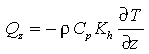
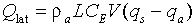
The vertical turbulent entrainment across the base of the mixed layer can deepen the
mixed layer and contributes a term Q
to equation (1):
![]() (8)
(8)
where  T is the temperature jump
across the mixed layer base. Estimation of Q
requires a measure of W
T is the temperature jump
across the mixed layer base. Estimation of Q
requires a measure of W and T. Following McPhaden
[1982], W = W
> 0 where
and T. Following McPhaden
[1982], W = W
> 0 where
 (9a)
(9a)
The time rate of change of mixed layer depth is h/t and W is the vertical velocity in the
thermocline just below the base of the mixed layer. Requiring W > 0 is necessary
to satisfy the condition that entrainment can only cool the mixed layer. Assuming
negligible heat flux across isotherms and ignoring horizontal advective terms in the
thermocline, the entrainment velocity can be approximated by:
is the vertical velocity in the
thermocline just below the base of the mixed layer. Requiring W > 0 is necessary
to satisfy the condition that entrainment can only cool the mixed layer. Assuming
negligible heat flux across isotherms and ignoring horizontal advective terms in the
thermocline, the entrainment velocity can be approximated by:
 (9b)
(9b)
The depth of the 20°C isotherm (h )
is used to represent thermocline motions, since this isotherm is usually just below the
mixed layer in the low-pass-filtered time series (Figure 5).
)
is used to represent thermocline motions, since this isotherm is usually just below the
mixed layer in the low-pass-filtered time series (Figure 5).
The appropriate temperature difference T at
the base of the mixed layer is difficult to specify a priori. However, we estimated this
temperature by computing the linear regression between -CW and Q. The correlation coefficient was 0.64, and the
regression coefficient (1.7°C) was used for T
in equation (8). The mean temperature gradient below the
mixed layer was about 0.1°C m, so this average value
of T represents upwelling from about 20 m
deeper than h.
Our estimates of W and T were used to compute Q (Figure 6c).
This time series is well correlated with the mixed layer heating (correlation coefficient
of 0.64 as noted above) and has a standard deviation of 22 W m. Both positive and negative values of Q are included in Figure
6c and the correlation, to take into account the fact that the local winds are
almost always upwelling favorable. Thus one can consider the fluctuations of Q to be superimposed on a mean cooling, with
positive values of Q representing a
reduction in this cooling.
Variability in Q was not
significantly correlated with the local zonal wind speed. The largest fluctuations in Q were between early July and mid-September 1986
and between November 1986 and January 1987. In both cases the change in Q was almost 85 W m and was in phase with the fluctuations of mixed layer
heating. Local wind variations during this period were small.
Recent observational studies of near equatorial turbulence at 140°W [Gregg
et al. 1985; Peters
et al., 1987; Moum
et al., 1989] indicate that the turbulent heat flux at the base of the
mixed layer is similar in magnitude to the atmospheric heat flux at the ocean
surface. Turbulent processes are not directly measured by the equatorial moorings;
hence the turbulent heat flux can be only estimated using a parameterization
of the mixing processes. We assume that the turbulent heat flux is down the
temperature gradient and represented by an eddy coefficient, K :
:
 (10)
(10)
Relating the eddy coefficient to a single parameter of the mean field provides
the simplest parameterization of turbulent mixing. Following Pacanowski
and Philander [1981], we assume that K is a function of the Richardson number Ri and write:
![]() (11)
(11)
with
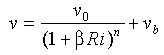
where n,  ,
,  , K
, K ,
and are
empirical constants, g = 9.8 m s is the
gravitational acceleration, and = 8.75 × 10
,
and are
empirical constants, g = 9.8 m s is the
gravitational acceleration, and = 8.75 × 10 (T+9) (°C) is the
thermal expansion coefficient. The temperature T is in degrees Celsius.
(T+9) (°C) is the
thermal expansion coefficient. The temperature T is in degrees Celsius.
The parameterization in (11) is the form of vertical
mixing used in several recent numerical general circulation model simulations
of the tropical oceans [Philander,
1990]. Peters
et al. [1987] have shown on the basis of turbulence measurements at
140°W that this functional form for K
(Ri) yields reasonable agreement with equatorial measurements for Ri
> 0.5; however, the empirical constants in (11)
derived from the data differ in magnitude from those used in the numerical models.
These constants are likely to vary with location and time as well as with the
vertical resolution over which the gradients are calculated. Hence for our study
we assumed the constants given by Pacanowski
and Philander [1981]: n = 2,
= 5,
= 5 × 10 m s ,
= 1 × 10 m
s, and K
= 1 × 10
s ,
= 1 × 10 m
s, and K
= 1 × 10 m
s.
m
s.
The vertical diffusive heat flux was computed from the mooring data in Figure 5 using (10) and (11). Vertical gradients of temperature and velocity were estimated by centered differences on the 5-m gridded data. Figure 7 shows the mixed layer depth and the Richardson number below the mixed layer. The seasonal variations of the Richardson number was similar in 1986 and 1987; Ri was relatively high in August-September and low in May-June. The small Ri in May-June is clearly associated with the occurrence of strong shear below the mixed layer as the Equatorial Undercurrent (EUC) intensifies. The high Ri in August-September corresponds to the deepening of the EUC and the reduction in near surface shear. When the mixed layer is deep the Richardson number tends to be large. However, in March-April 1988 the largest Richardson numbers occurred at a time when the mixed layer was very shallow. At that time the near-surface shear was small and the vertical temperature gradient was large as cool surface water appeared in the eastern equatorial Pacific.
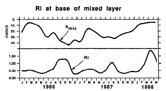
Fig. 7. Low-pass-filtered (91-day Hanning filter) time series of the mixed layer
depth h and Richardson number Ri
at the base of the mixed layer at 0°, 110°W, estimated as described in the text.
The turbulent diffusion of heat out of the mixed layer is shown in Figure 6d. As can be expected, the variations in Ri have a strong influence on the estimated heat flux. High Ri corresponds to small vertical heat flux, and vice versa. Seasonal changes in mixed layer temperature are well correlated with the vertical heat flux except in spring 1988. In fall 1986 and spring 1987, the large mixed layer heating corresponded to decreased turbulent flux out of the mixed layer. Similarly, the decreased heating in November-December 1986 and May 1987 corresponded to increased downward turbulent flux. Spring 1988 remains anomalous, since the high Ri at that time suppresses the turbulent flux; vertical heat flux out of the mixed layer decreased at the same time that the layer was cooling.
On average, the vertical turbulent diffusion exported about 130 W m to the deep ocean with rms fluctuations of 40 W m. This flux nearly balanced the net surface flux (115 W m) into the mixed layer (Figure 4),
suggesting that vertical diffusion is probably the dominant internal oceanic process
controlling the annual average mixed layer temperature in the eastern Pacific.
Up to now, the individual contributions of Q, Q, Q and Q to the mixed layer temperature change have been estimated and no single term
has been found which accounts for the observed variations of Q. Estimation of the remaining terms in equation (1), meridional advection and diffusion, require
off-equatorial information. Such data are not available continuously throughout the study
period ( Figure 1) because of deployment schedules and
instrument failures. Coverage is best in boreal spring of each year and these records are
discussed in the next section. First, however, we consider how well the sum of the terms
available throughout the entire record can balance the heating.
Figure 6e shows the comparison of the sum of the
surface heat flux, penetrative radiation, zonal advection, entrainment and vertical
diffusion (Q = Q + Q + Q + Q) and the observed mixed layer heating (Q). Over the entire 29-month record the
correlation coefficient between the two series was 0.71; limiting the record to 24 months
in 1986-87 increases the correlation to 0.80. Both of these correlations are significant
at the 95% level. The linear regression coefficient (1.1) between the two complete series
indicates that the fluctuations in Q are about 10% larger than those observed in surface heating. The offset
between the two series showed that the mean surface heating was about 30 W m larger than Q. Thus an additional heating source
(perhaps meridional diffusion) is required to balance these terms.
Observed and computed heating agreed reasonably well in 1986. During the initial
development of warm conditions in the eastern Pacific in August through November 1986
[MH], the mixed layer was relatively deep and was warming by up to nearly 100 W m. This heat was provided by the net solar radiation (which
was enhanced at that time by the semiannual cycle in Q and the reduced Q associated with the deep mixed layer), and
variations in all the oceanic terms. Changes in latent heat flux do not appear to
contribute to this warming. The large increase in heating in mid-September 1986 was
associated with reduced oceanic cooling as the zonal advection was near zero, vertical
entrainment was reduced, and vertical diffusion was near its minimum.
The phase of the seasonal cycle from February through July 1987 was also rather well
represented by the computed heat flux terms. Ignoring the rapid rise in January, the
general spring warming in 1987 required about 50 W m
in February. This heat was provided by the net solar radiation and reduced vertical
diffusion. Reduced zonal advective cooling is nearly balanced by increased entrainment.
The subsequent cooling in May-July appears to result primarily from a large increase in
vertical turbulent diffusion out of the mixed layer. This diffusion and increased
entrainment is sufficient to counteract the increased mixed layer heating associated with
zonal advection.
Relatively large (>50 W m) discrepancies between
the surface heating and the heat flux occur throughout the record although the phase of
the two terms generally agree. In January 1987 the observed mixed layer heating was nearly
60 W m larger than the estimated heat flux into the
mixed layer. In May 1987 the estimated cooling was nearly 100 W m too large. The period March-May 1988 also remains
anomalous. At that time changes in heating and heat flux were out of phase. As the mixed
layer cooled by about 10 W m (and SST dropped nearly
8°C), the heat flux was trying to warm the ocean by up to 50 W m. This period is considered in the context of boreal spring
1986 and 1987 in the next section.
During boreal spring of each of the years considered the data coverage off the equator at 110°W was more extensive (Figure 1). These years provide interesting contrasts (Figure 2): spring 1986 was relatively normal, spring 1987 experienced the warmest eastern Pacific SST of the ENSO event, and in spring 1988 the subsequent cold event began. The enhanced data coverage from the off-equatorial mooring allows a more complete description of these periods and estimation of additional terms in the heat budget.
Figure 8 shows the wind, SST, and thermocline depth time series for the six month periods December though May of 1985-1986, 1986-1987, and 1987-1988. These periods are referred to below as 1986, 1987, and 1988. The wind time series are represented by arrows which point in the direction toward which the wind is blowing (north is toward the top of the page) and whose length is proportional to speed. These sticks are 3-day subsamples of the daily data which have been filtered with a 21-day Hanning low pass filter. Temperature and thermocline depth time series show both daily averaged (thin line) and 21-day Hanning low-pass-filtered (heavy line) data. The 18°C isotherm is used to represent the thermocline depth, since the 20°C isotherm surfaces at the equator in spring 1988 (Figure 2). Note that the temperature and depth scales are correct for the equatorial location. The time series of SST and 18°C depth at the other latitudes are offset by the amounts given in the figure caption.
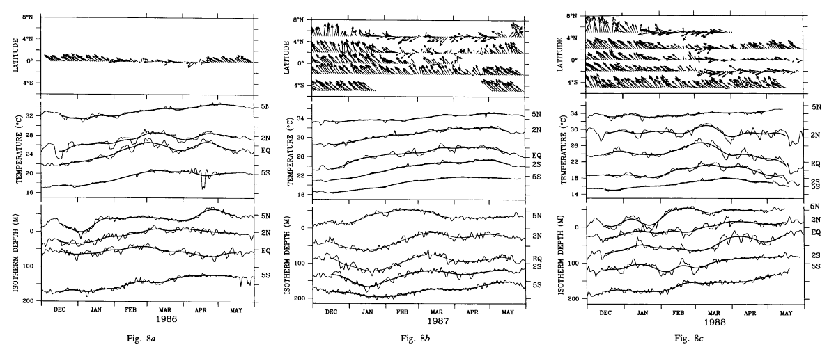
Fig. 8. Time series of the winds, SST, and depth of the 18°C isotherm for boreal
spring of (a) 1986, (b) 1987, and ( c) 1988 at the latitudes
indicated along 110°W. Wind sticks point in the direction toward which the wind is
blowing. The length of the sticks is such that 20 m s
is equivalent to the monthly tick marks on the time axis. For SST and 18°C depth, the
light line indicates the daily data and the heavy line indicates a 21-day Hanning low-pass
filter. The 5°S SST in 1986 is actually the 20-m temperature record. The SST and 18°C
depth scales are correct for the equatorial time series. The SST time series at the other
latitudes have been offset as follows: 5°N and 2°N are offset by 6°C and 3°C for all 3
years shown, 2°S is offset by -3°C in 1987 and by -6°C in 1988, and 5°S is offset by
-6°C in 1986 and 1987 and by -10°C in 1988. The 18°C time series offsets are the same
in all years: 5°N is offset by -125 m, 2°N by -50 m, 2°S by 50 m, and 5°S by 75 m.
The meridional distribution of SST change was similar in 1986 and 1987; however, the mean temperature was about 1.5°C warmer in 1987. Warming began in January and occurred nearly simultaneously at all latitudes sampled. Maximum temperature was in March-April, when SST near the equator was about 3°C higher than the December value. In 1988, the SST change south of 5°N was considerably more irregular than in the other 2 years. SST warmed in January-February but began to decrease in mid-March. Equatorial SST fell from a high of 27°C in March to 19°C in May. At 5°N the seasonal SST change was nearly normal.
Wind time series showed the seasonal movement of the intertropicl convergence zone (ITCZ) and the decrease in the Southeast trades near the equator. The wind vectors began turning first near 5°N and then moved towards the equator. In all years, periods of northerly winds occurred on the equator; in 1988 these winds extended to 2°S. In April-May of 1988, strongly divergent winds developed about the equator as the anomalously cool water appeared. Hayes et al. [1989b] suggest that this divergence was in part a response to the SST gradient.
Thermocline depth tended to decrease throughout the spring period of all years. This low-frequency trend was most apparent at 5°S, where warmest SST occurred while the thermocline was shoaling. Near the equator the monthly variability is more pronounced and there is little correlation of SST and thermocline variations on this time scale.
There was a pronounced deepening of the thermocline in January 1987 (about
50 m) which appears to be equatorially trapped. Empirical orthogonal function
(EOF) analysis [Davis,
1976] of the surface dynamic height time series derived from the moored
temperature measurements using a latitude dependent temperature-salinity relation
captured this equatorially symmetric variability in the first mode, which accounted
for 66% of the total variance. The meridional structure function for this mode
near the equator is well fit by the structure of a first baroclinic mode equatorial
Kelvin wave (Figure 9) assuming a phase speed
C = 2.1 m s [Hayes
and Halpern, 1984]. This Kelvin signal was noted in MH, who attributed
it to wind variability in the western Pacific in November-December. This interpretation
was supported by Delcroix
et al. [1991], who used Geosat satellite altimeter measurements to trace
this sea level signal across the Pacific. The signal is apparent in the variations
of the deeper zonal currents (e.g., 120 m current in Figure
10); however, the surface zonal velocity shows no indication of this event.
The weak surface signal is consistent with the effects of wave mean flow interactions
[McPhaden
et al., 1987] and with general circulation model (GCM) studies of the
propagation of Kelvin pulses [Geise
and Harrison, 1990].
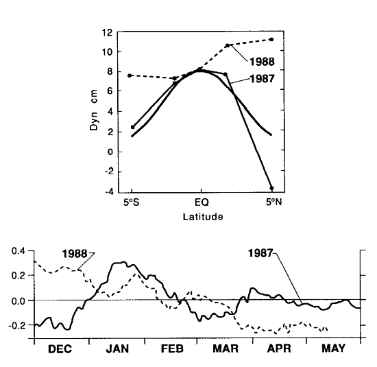
Fig. 9. Meridional structure functions and time series of the first EOF of surface
relative to 300 dbar dynamic height constructed from the temperature time series along
110°W in 1987 and 1988. For comparison the meridional structure of a first-vertical-mode
equatorial Kelvin wave with a phase speed of 2.1 m s
is also shown.
In 1988 the 18°C isotherm rose about 75 m from December to May and nearly broke the surface. The mixed layer was very thin (Figure 5) or nonexistent. This shoaling was not trapped to the equator. The structure function of the first EOF (which explained 70% of the variance) of surface dynamic height relative to 300 dbar (Figure 9) was fairly uniform from 5°N to 5°S and the time series showed the sea level decrease which accompanied the thermocline rise. This drop in sea level was about 5 dyn cm at 5°N.
A prominent feature of the zonal surface current was the onset of eastward surface
current each year (Figure 10). Persistent eastward flow
began in mid-March, after SST had warmed. The systematic change was confined to near the
surface. There was not a consistent pattern at 120 m. Strongest eastward near surface
zonal speed was in 1986 (about 50 cm s in April),
weakest was in 1987.
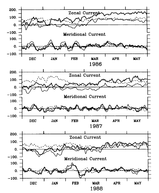
Fig. 10. Time series of zonal and meridional velocity on the equator at 110°W at depths of 10 m (light line), 45 m (heavy line), and 120 m (dashed line) for boreal spring of 1986, 1987, and 1988. Units of velocity are centimeters per second.
Meridional velocity exhibited the 20- to 30-day variability associated with the tropical instability oscillations in the eastern Pacific [Halpern et al., 1988]. This signal was most apparent in December-March 1986 and was again seen during this period in 1988. During the 1987 warm event the instability oscillations were weaker; this weakening was also noted during the 1982-1983 warm event [Philander et al., 1985].
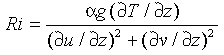
The off equatorial thermal measurements available in boreal spring allow estimation of the meridional terms in the mixed layer temperature equation (1).
![]() (12)
(12)
 (13)
(13)
where
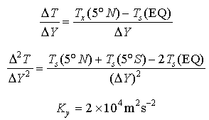
where the SST at latitude Y is T(Y) and Y = 5°.
The form of the meridional diffusive heat flux (equation
13) is the same as that used in numerical models of the tropical ocean [Philander
and Pacanowski, 1980]. The value of the eddy coefficient K
was chosen based on the results of Hansen
and Paul [1982] and Bryden
and Brady [1989]. These studies estimated meridional heat transport
associated with the tropical instability waves and inferred an eddy coefficient.
This coefficient likely changes seasonally and interannually (in boreal spring
and during ENSO warm events the instability waves are weaker or disappear) and
is probably a function of latitude. In the estimation of Q
these possible variations were ignored. The value of K
used corresponds to the Hansen
and Paul [1982] estimate and is about a factor of three larger than
the mean value at 20 m found by Bryden
and Brady [1989].
The meridional temperature gradient in equation (11) was estimated from the moored data by differencing the 5°N and equatorial records. This probably overestimates the actual gradient at the equator. The second derivative was obtained by second differencing the 5°N, 0°, and 5°S records. In order to obtain as long a record as possible in spite of data gaps, the time series were filtered using only a 45-day low pass Hanning filter instead of the 91-day filter used in Figure 6. The 45-day filter length was chosen in order to reduce the influence of the tropical instability waves which have an average period of about 20 days [Halpern et al. 1988] which is close to the zero of the Hanning filter. The effects of these waves are then included in the eddy flux.
Time series of the mixed layer heating, Q;
the meridional advective heat flux, Q;
the meridional diffusive heat flux, Q;
and sum of all heat flux terms on the right hand side of equation
(1), Q ,
are shown in Figure 11 for all three
years.
,
are shown in Figure 11 for all three
years.
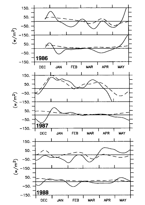
Fig. 11. The top panel for each year shows time series (45-day low-pass Hanning
filter) of Q (dashed) and Q (solid; see text for definition).
The bottom panel for each year shows meridional diffusive heat flux Q (dashed) and meridional advective heat flux Q (solid). Records for boreal spring 1986, 1987,
and 1988 are shown.
The meridional diffusive heat flux had a characteristic pattern each year. It was
largest in December, weakest in March, and increased again in May. This pattern simply
reflects the strength of the equatorial cold tongue and hence the meridional curvature of
SST at the equator. Maximum estimated magnitude was about 50 W m. The diffusive heat flux always tends to warm the equator.
Estimates of the meridional advective heat flux can be quite large because
of the strong front just north of the equator. The resolution provided by the
moorings is not adequate to accurately resolve this front and establish the
meridional temperature gradient right on the equator. It is likely that our
estimates of Q are often
too large. Adding this term improves the agreement between the mixed layer heating
and the heat flux into the mixed layer during the warming (December-January)
of all three years. Interestingly, the rapid rise in temperature in January
1987 which appears to be associated with the passage of the Kelvin wave event
(Figure 9) is seen in the meridional but not
the zonal advective heat flux. Geise
and Harrison [1990] speculated that Kelvin pulses can modify the background
instability wave field in the eastern equatorial Pacific and lead to relatively
large changes in meridional velocity even though the Kelvin signal itself has
no meridional velocity component. Perhaps this effect is responsible for the
nearly 100 W m meridional heat advection
in January 1987.
A major discrepancy between the temperature change and the estimated heat flux
developed in May 1986 (compare Figure 6e and 11). At that time the cold tongue was recovering and the mixed
layer was deepening. A weak southward velocity led to a large apparent warming of 150 W m. The discrepancy in May 1987 continued to be present even
with inclusion of meridional terms. The meridional advection enhanced the erroneous
cooling seen in Figure 6 e. It appears that during
the period when the equatorial front is intensifying, the moored data, with coarse spacial
resolution, do not adequately resolve the fluctuations.
Time series of surface wind and upper ocean temperature and velocity have been used to describe the variations of the mixed layer temperature for the period January 1986 to June 1988. This period included the development of the 1987 ENSO warm event and the subsequent cooling. Mixed layer heating was compared to estimates of the surface heat flux using a combination of the moored measurements and climatology. Oceanic heat transports were parameterized and estimated from the moored measurements. Given the uncertainties in all the estimates and the approximations involved in the parameterizations, the agreement between the changes in mixed layer temperature and the net heating of this layer is remarkably good (Figures 6e and 11). The major features of the temperature changes in 1986 and through the first half of 1987 are reasonably well represented. However, in late 1987 and in spring 1988 temperature change and heat flux were out of phase. In particular, the cooling which followed the 1987 warm event was not well described. During this period the mixed layer was very shallow and the assumptions used in the calculations were not valid.
Although no single term in the temperature (1) dominated the mixed layer heating, the
most important terms in the mean balance were the net incoming surface heat flux and the
vertical flux out the bottom of the mixed layer. Both the penetrative solar radiation (Q) and the vertical turbulent flux (Q) contributed to the latter. The mean net heat
flux at the surface was 165 W m and the sum of Q and Q was 180 W m; thus the mean heat input at
the ocean surface nearly balances the vertical flux through the mixed layer.
Fluctuations in Q were also quite
important in the variability of the mixed layer heat content. A decrease in the vertical
turbulent flux out of the mixed layer contributed about half of the heat flux change which
led to the warming in September-October 1986, and an increase in Q could account for nearly all of the cooling in
May 1987. Overall the vertical turbulent heat flux variation was well correlated with the
mixed layer heating (r = 0.5), and the rms amplitude of the Q and Q fluctuations were comparable.
Vertical entrainment of cool water into the mixed layer also plays an important role in
the variability of the mixed layer temperature (Figure 6c).
This term is well correlated with Q
(0.64) and inclusion of Q in Q increases the correlation coefficient
between Q and Q from 0.5 to 0.7. Our estimate of the
entrainment velocity is quite crude and fails particularly when the mixed layer is very
shallow, such as in spring 1988. From March to May 1988 the 20°C isotherm rose 50 m and
in the daily averaged time series actually broke the surface (Figure
2). This upwelling likely contributed substantially to the SST cooling observed at
that time. However, with the data available there is no way to accurately estimate this
vertical advective cooling. Figure 6e suggests that
about -60 W m would be required to bring Q and Q into balance during this period. The mean
upwelling of the thermocline from March to May was about 1 m d (1.1 × 10 m s), and the temperature change from the surface to 5 m (our
minimum mixed layer depth) was 1°C. Thus, from (8) the
vertical entrainment cooling could easily contribute -50 W m.
Zonal advection was a significant contribution to the heat flux variability.
The seasonal cycle of the surface current [Halpern,
1987; McPhaden
and Taft, 1988] leads to advective warming in boreal spring and cooling
in the fall. The total change between the two seasons was about 75 W m
in 1986. However, the relation of the advective heat flux to the mixed layer
temperature change is not simple. Maximum SST and eastward surface current were
nearly in phase; hence the springtime warming of the mixed layer occurred before
the surface current reversed. Thus on seasonal time scales, the advective heat
flux tended to be out of phase with the warming. During the onset of the 1986-87
ENSO warm event in the eastern Pacific in late 1986, reduced westward surface
current contributed to the warming as suggested in MH. However, the seasonal
cycle persisted through the 1987 warm event, and the increasing mixed layer
temperature in January-March 1987 was opposed by advective cooling. The large
heating in January 1987 coincided with the deepening of the thermocline associated
with the arrival of a Kelvin pulse (Figures 8b
and 9). This signal, however, had little surface
zonal velocity expression and hence was not apparent in the zonal heat advection.
Meridional advection and diffusion were examined during December to May of the 3 years considered. Since meridional SST gradients are generally weakest during boreal spring, the overall importance of the meridional terms may be underestimated in our results. On the other hand, the eddy coefficient used was derived by Hansen and Paul [1982] based on measurements in boreal summer and fall when the tropical instability waves are largest. Hence this coefficient is likely to be too large.
The meridional advective heat flux was generally small, perhaps because the
site is directly on the equator. This term can, however, contribute to the intraseasonal
fluctuations. For example, meridional advection supplied nearly 100 W m
in January 1987 during the passage of the Kelvin wave event. As noted above,
this contribution from the meridional velocity is, presumably, indicative of
the effects which the Kelvin signal has on the instability waves. In the model
studies [Geise
and Harrison, 1990] the magnitude of the meridional term depends critically
on the amplitude and phase of the instability waves at the time of the event.
Meridional diffusion is highly parameterized in (10).
However, if the diffusive heat flux is proportional to the meridional curvature of the
temperature field, then the phase of this term is reasonably well represented in our
analysis. Meridional diffusion appears to be important in the seasonal heating. In
December-January this term contributes 40-50 W m at
the time when the mixed layer is most rapidly warming. In 1986 and 1988 this meridional
term was crucial in order to obtain a near balance in the January heat budget. In
February-March of each year the equatorial cold tongue nearly vanished at 110°W and the
temperature curvature was a minimum. At this time the instability waves disappeared and
the diffusive heat flux was near zero. In April-May the equatorial cold tongue returned
and meridional diffusion tended to warm the equator. This warming is counter to the
general cooling trend in the mixed layer and slows the development of the cold tongue.
In summary, the picture which emerges from this analysis of the eastern equatorial Pacific heat budget is one in which many heat flux terms are important. The local change in mixed layer temperature cannot be ascribed to any single process for the duration of the record. The relatively simple correlations between SST changes and local wind on seasonal and interannual time scales (Figure 3) is the result of a complicated interaction of variations of surface fluxes and oceanic processes. Our conclusion is similar to that of Weingartner and Weisberg [1991], who found that the seasonal upper ocean heat budget in the equatorial Atlantic was also the result of the interplay of several terms. Our analyses relied heavily on parameterizations of both the atmospheric flux terms and the oceanic processes. A more quantitative study of the mixed layer heat budget will require more accurate measurements, and some improvement of the parameterizations, of these terms.
Acknowledgments. We would like to thank C. Deser for providing the COADS data set and her analysis of climatological surface parameters. We are grateful for the assistance of L. Mangum, N. Soreide, and L. Stratton in the analysis and the computations. This work was supported, in part, by the Equatorial Pacific Ocean Climate Studies (EPOCS) Project of ERL/NOAA through grants to PMEL (S.P.H., M.J.M.) and JISAO, University of Washington (P.C.). NOAA Pacific Marine Environmental Laboratory contribution 1160.
Battisti, D., Dynamics and thermodynamics of a warming event in a coupled ocean/atmosphere model, J. Atmos. Sci., 45, 2889-2919, 1988.
Bryden, H.L., and E.L. Brady, Diagnostic model of the three dimensional circulation in the upper equatorial Pacific Ocean, J. Phys. Oceanogr., 15, 1255-1273, 1985.
Bryden, H.L., and E.C. Brady, Eddy momentum and heat fluxes and their effect on the circulation of the equatorial Pacific Ocean. J. Mar. Res., 47, 55-79, 1989.
Cane, M.A., and S.E. Zebiak, A theory for El Nińo and the Southern Oscillation, Science, 228, 1085-1087, 1985.
Davis, R.E., Predictability of sea surface temperature and sea level pressure anomalies over the North Pacific Ocean, J. Phys. Oceanogr., 6, 249-266, 1976.
Delcroix, T., J. Picaut, and G. Eldin, Equatorial Kelvin and Rossby waves evidenced in the Pacific Ocean through GEOSAT sea level and surface current anomalies, J. Geophys. Res., 96, suppl., 3249-3262, 1991.
Deser, C., Meteorological characteristics of the El Nińo/Southern Oscillation Phenomenon, Ph.D. Dissertation, Univ. of Wash., Seattle, 1989.
Dobson, J.W., and S.D. Smith, Bulk models of solar radiation at sea, Q. J. Roy. Meteor. Soc., 114, 165-182, 1988.
Enfield, D.B., Zonal and seasonal variability of the equatorial Pacific heat balance, J. Phys. Oceanogr., 16, 1038-1054, 1986.
Esbensen, S.K., and V. Kushnir, The heat budget of the global ocean: An atlas based on estimates from marine surface observations, Rep. 29, Clim. Res. Inst., Oreg. State Univ., Corvallis, 1981.
Giese, B.S., and D.E. Harrison, Aspects of the Kelvin wave response to episodic wind forcing, J. Geophys. Res., 95, 7289-7312, 1990.
Gregg, M.C., H. Peters, J.C. Wesson, N.S. Oakey, and T.J. Shay, Intensive measurements of turbulence and shear in the equatorial undercurrent, Nature, 318, 140-144, 1985.
Halpern, D., Observations of annual and El Nińo thermal and flow variations at 0°, 110°W and 0°, 95°W during 1980-1985, J. Geophys. Res., 92, 8197-8212, 1987.
Halpern, D., S. Hayes, A. Leetmaa, D. Hansen, and G. Philander, Oceanographic observations of the 1982 warming of the tropical Pacific, Science, 221, 1173-1175, 1983.
Halpern, D., R.A. Knox, and D.S. Luther, Observations of 20-day period meridional current oscillations in the upper ocean along the Pacific equator, J. Phys. Oceanogr., 18, 1514-1534, 1988.
Hansen, D., and C.A. Paul, Genesis and effects of long waves in the equatorial Pacific, J. Geophys. Res., 89, 10,431-10,440, 1982.
Hayes, S.P., and D. Halpern, Correlation of upper ocean currents and sea level in the eastern equatorial Pacific, J. Phys. Oceanogr., 10, 633-635, 1984.
Hayes, S.P., M.J. McPhaden, and A. Leetmaa, Observational verification of a quasi-real-time simulation of the tropical Pacific Ocean, J. Geophys. Res., 94, 2147-2157, 1989a.
Hayes, S.P., M.J. McPhaden, and J.M. Wallace, The influence of sea surface temperature upon surface wind in the eastern equatorial Pacific: Weekly to monthly variability, J. Clim., 2, 1500-1506, 1989b.
Hayes, S.P., L.J. Mangum, J. Picaut, A. Sumi, and K. Takeuchi, TOGA-TAO: A moored array for real-time measurements in the tropical Pacific Ocean. Bull. Am. Meteorol. Soc., 72, 339-347, 1991.
Ivanov, A., Oceanic absorption of solar radiation, in Modelling and Prediction of the Upper Layers of the Ocean, edited by E.B. Kraus, pp. 47-71, Pergamon, New York, 1977.
Large, W.G., and S. Pond, Open ocean momentum flux measurements in moderate to strong winds. J. Phys. Oceanogr., 11, 324-336, 1982.
Liu, W.T., and P.P. Niiler, The sensitivity of latent heat flux to the air humidity approximations used in ocean circulation models, J. Geophys. Res., 95, 9745-9753, 1990.
Mangum, L.J., S.P. Hayes, and J.M. Toole, Eastern Pacific circulation near the onset of the 1982-1983 El Nińo, J. Geophys. Res., 91, 8428-8436, 1986.
McPhaden, M.J., Variability in the central equatorial Indian Ocean, Part II. Oceanic heat and turbulent energy balance, J. Mar. Res., 40, 403-419, 1982.
McPhaden, M.J., and S.P. Hayes, Variability in the eastern equatorial Pacific Ocean during 1986-1988, J. Geophys. Res., 95, 13,195-13,208, 1990.
McPhaden, M.J., and S.P. Hayes, On the variability of winds, sea surface temperature, and surface layer heat content in the western equatorial Pacific, J. Geophys. Res., 96, suppl., 3331-3342, 1991.
McPhaden, M.J., and B.A. Taft, On the dynamics of seasonal and intraseasonal variability in the eastern equatorial Pacific Ocean to a westerly wind burst in May 1986, J. Geophys. Res., 93, 10,589-10,603, 1988.
McPhaden, M.J., J.A. Proehl, and L.M. Rothstein, On the structure of low frequency equatorial waves, J. Phys. Oceanogr., 17, 1555-1559, 1987.
Meyers, G., J.R. Donguy, and R.K. Reed, Evaporative cooling of the western equatorial Pacific Ocean by anomalous winds, Nature, 323, 523-526, 1986.
Milburn, H.B., and P.D. McLain, ATLAS--A low cost satellite data telemetry mooring developed for NOAA's climate research mission, in Proceedings MDS 1986, Marine Data Systems International Symposium, 393-396, Marine Technology Society, Washington, D.C., 1986.
Moum, J.N., D.R. Caldwell, and C.A. Paulson, Mixing in the equatorial surface layer and thermocline, J. Geophys. Res., 94, 2005-2021, 1989.
Pacanowski, R., and S.G.H. Philander, Parameterization of vertical mixing in numerical models of tropical ocean, J. Phys. Oceanogr., 11, 1443-1451, 1981.
Peters, H., M.C. Gregg, and J.M. Toole, On the parameterization of equatorial turbulence, J. Geophys. Res., 92, 5481-5488, 1987.
Philander, S.G.H., El Nińo, La Nińa, and the Southern Oscillation, 289 pp., Academic, San Diego, Calif., 1990.
Philander, S.G.H., and W.J. Hurlin, The heat budget of the tropical Pacific in a simulation of the 1982-83 El Nińo, J. Phys. Oceanogr., 18, 926-931, 1988.
Philander, S.G.H., and R.C. Pacanowski, The generation of equatorial currents, J. Geophys. Res., 85, 1123-1136, 1980.
Philander, S.G.H., D. Halpern, D. Hansen, R. Legeckis, L. Miller, C. Paul, R. Watts, R. Weisberg, and M. Wimbush, Long waves in the equatorial Pacific Ocean, EOS Trans. AGU, 66, 154, 1985.
Reed, R.K., On estimating insolation over the ocean, J. Phys. Oceanogr., 7, 482-485, 1977.
Reed, R.K., Heat fluxes over the eastern tropical Pacific and aspects of the 1972 El Nińo, J. Geophys. Res., 88, 9627-9638, 1983.
Stevenson, J.W., and P.P. Niiler, Upper ocean heat budget during the Hawaii-to-Tahiti Shuttle Experiment, J. Phys. Oceanogr., 13, 1894-1907, 1983.
Wallace, J.M., T.P. Mitchell and C. Deser, The influence of sea-surface temperature upon surface wind in the eastern equatorial Pacific: Seasonal and interannual variability, J. Clim., 2, 1492-1499, 1989.
Weare, B.C., Uncertainties in estimates of surface heat fluxes derived from marine reports over the tropical and subtropical oceans, Tellus, Ser. A, 41, 357-370, 1989.
Weare, B.C., P.T. Strub, and M.D. Samuel, Annual mean surface heat fluxes in the tropical Pacific Ocean, J. Phys. Oceanogr., 11, 705-711, 1981.
Weingartner, T.J., and R.H. Weisberg, A description of sea surface temperature and upper ocean heat variability in the central equatorial Atlantic, J. Phys. Oceanogr., in press, 1991.
Wyrtki, K., An estimate of equatorial upwelling in the Pacific, J. Phys. Oceanogr., 11, 1205-1214, 1981.