U.S. Dept. of Commerce / NOAA / OAR / PMEL / Publications
We used two data sets spanning the period 1946-1993 for this study: COADS Release 1 with the 1a standard extension, published by the NOAA Environmental Research Laboratories (Slutz et al., 1985; Woodruff et al., 1987, 1993), and a time series of Darwin SLP, Tahiti SLP, and Troup SOI provided by Dr. Grant Beard of the Australian Bureau of Meteorology. We used the Darwin and Tahiti data to check for consistency with the COADS SLP signals, and used COADS for the bulk of our work. We examined results using both SLP and SLP anomalies (SLPA), defined to be the departure of a particular month from the 1946-1993 monthly climatology. We investigated the effect of using other climatologies, including ones that leave out the ENSO periods, but the major results stay the same; only in periods of small SLPA can the choice of climatology lead to substantially different SLPA patterns.
The limitations of the COADS data for climate studies can be substantial and depend greatly on the variable(s) of interest. We shall not recapitulate the questions that have been raised in previous studies of SST and surface winds, particularly those concerned with identifying multi-decadal trends. Others have found the COADS SLP data to be useful for their studies. Barnett (1985) used COADS SLP for his principal component analysis. Wright et al. (1988), in particular, describe their efforts to scrutinize COADS SLP data. We feel that our SOI "validation" described in Section 3 further supports use of COADS data for this study. On the basis of this, we proceed with further work using the COADS SLP data.
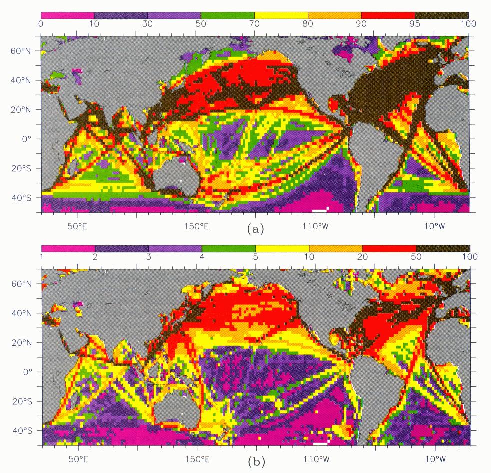
Whenever attempting to evaluate fields of variables from noisy and gappy data sets like COADS, however, the limits of the data distribution should be kept in mind. The data distribution (Figure 1a) shows that shiptracks and data-deficient regions characterize much of the world ocean. The amount of data is much more limited in the southern hemisphere, and the tropics are not well covered. Poleward of 30°S and 60°N there is very little data. The data coverage and the number of observations in each monthly averaged data point also shows substantial variation (Fig. 1b). We have no information regarding the calibration of different barometers, so the underlying "noise" level of our analyses in different regions is not clear.
Fig. 1. The distribution of the 1946-1993 COADS SLP data. a) Percentage of months in which each 2 × 2 degree grid point has data. b) Average number of observations used in calculating each monthly mean COADS SLP data point.
The composite maps presented in this paper are smoothed to highlight the larger scale features by filtering smaller scale temporal and spatial noise. After considerable experimentation, we decided to adopt the smoothing technique used in RC. For our purposes "RC smoothed" is defined as the following procedure: the spatial grid is filled using linear zonal interpolation to define values at points with no data; this is followed by a nine-point (18°) zonal binomial smoother and a seven-point (14°) meridional binomial smoother, after which a 3-month running mean is applied. The zonal smoother has a half power wavelength of 21°; the meridional smoother has a half power wavelength of 18°. Near land the spatial smoothers are reduced to the dimension that will not extend over land. This creates an inconsistency between the near-boundary and mid-ocean smoothing, and boundary gradients will tend to be sharper than mid-ocean gradients due to the reduced smoothing.
Note that this smoothing procedure will not move the location of extrema under most circumstances, but will reduce their amplitudes. Were there better data coverage, so that the smoothing could be reduced, one might find regions of substantially greater gradient than seen here. It is important to note that all of the major features of the composite can be seen clearly in unsmoothed maps. Figure 2a-c shows a typical composite month using various spatial smoothers. More examples of minimally smoothed results are given in Larkin and Harrison (1996).
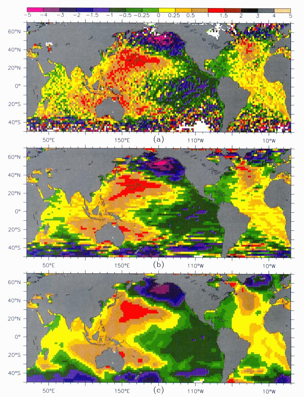
Fig. 2. The December Year(0) SLPA El Nińo composite (see section 4) using different spatial smoothers. a) No spatial smoothing. Note the non-uniform shading intervals, so that variability in the tropics can be seen. b) The same field with gaps filled via linear zonal interpolation, and smoothed via a zonal triangle of ten degree width. c) The same months smoothed by application of the RC smoother (see section 2). All composite results presented hereafter use this latter filling and smoothing.
The standard deviation statistics of this data set deserve some scrutiny and are used in Section 4. Figure 3 shows standard deviations computed over the 1946-1993 period, after the data has been RC-smoothed (above): Fig. 3a of the full (SLP) data set, Fig. 3b of the climatological seasonal march only, and Fig. 3c of SLPA only (climatological monthly means removed). The contour interval is 1 mb with the addition of the 0.5-mb contour to better show the structure of the variability in the tropics.
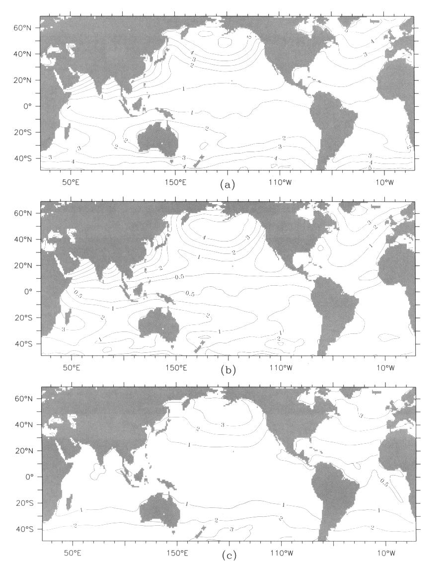
Fig. 3. Standard deviations of the RC smoothed 1946-1993 monthly COADS SLP data. The contour interval is 1 mb with the addition of the 0.5 mb contour to show structure in the tropics. a) standard deviation of SLP over the entire record. b) standard deviation of the monthly mean SLP climatology. c) standard deviation of SLP anomaly (monthly climatology removed) over the entire record.
The standard deviation of the full data set shows northern hemisphere maxima of 5 to 6 mb off the Aleutian Islands, off of Iceland-Greenland, along the coast near the Persian Gulf, and across the Indian subcontinent continuing on to Korea. The coastal maxima are expected due to the above mentioned smoothing limitations near boundaries. Except off Madagascar, the standard deviation is less than 2 mb until about 20°S. South of 20°S, it increases to a maximum of about 5 mb.
The pattern of the standard deviation of the seasonal march looks very much like that of the full data set north of 10°N. There are very small values (0.5 to 1 mb) over much of the tropics. South of 20°S the values stay small (1 to 2 mb), in contrast to those of the full standard deviation. In the northern hemisphere, the seasonal cycle accounts for a significant amount of the total variability in this monthly mean data set.
The standard deviation of the monthly mean anomalies has a different pattern from either that of the seasonal march or full data set. There is a broad tropical (20°S to 20°N) band of values near unity, and poleward of this the variance is largely an increasing function of latitude to about 4 mb at 50° from the equator. Away from the monsoon areas, the non-seasonal variations are found to be greater than the seasonal variations. In temperate northern hemisphere latitudes the seasonal and non-seasonal variance are similar in magnitude.
Return to previous section or go to next section