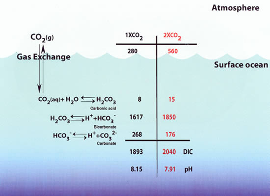
Figure 1. Schematic diagram of the carbon dioxide (CO![]() )
system in seawater. The 1 x CO
)
system in seawater. The 1 x CO![]() concentrations
are for a surface ocean in equilibrium with a pre-industrial atmospheric
CO
concentrations
are for a surface ocean in equilibrium with a pre-industrial atmospheric
CO![]() level of
280 ppm. The 2 x CO
level of
280 ppm. The 2 x CO![]() concentrations
are for a surface ocean in equilibrium with an atmospheric CO
concentrations
are for a surface ocean in equilibrium with an atmospheric CO![]() level
of 560 ppm. Current model projections indicate that this level could be reached
sometime in the second half of this century. The atmospheric values are in
units of ppm. The oceanic concentrations, which are for the surface mixed
layer, are in units of µmol kg
level
of 560 ppm. Current model projections indicate that this level could be reached
sometime in the second half of this century. The atmospheric values are in
units of ppm. The oceanic concentrations, which are for the surface mixed
layer, are in units of µmol kg![]() .
.
Figure 2. The Global Survey of CO![]() in
the Ocean: cruise tracks and stations occupied between 1991 and 1998.
in
the Ocean: cruise tracks and stations occupied between 1991 and 1998.
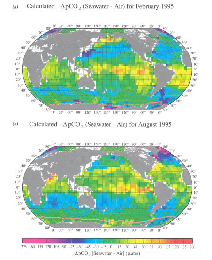
Figure 3. Distribution of climatological mean sea-air pCO![]() difference
(
difference
(![]() pCO
pCO![]() )
for the reference year 1995 representing non-El Niño conditions in February
(a) and August (b). These maps are based on about 940,000 measurements of
surface water pCO
)
for the reference year 1995 representing non-El Niño conditions in February
(a) and August (b). These maps are based on about 940,000 measurements of
surface water pCO![]() from
1958 through 2000. The pink lines indicate the edges of ice fields. The yellow-red
colors indicate regions with a net release of CO
from
1958 through 2000. The pink lines indicate the edges of ice fields. The yellow-red
colors indicate regions with a net release of CO![]() into
the atmosphere, and the blue-purple colors indicate regions with a net uptake
of CO
into
the atmosphere, and the blue-purple colors indicate regions with a net uptake
of CO![]() from
the atmosphere. The mean monthly atmospheric pCO
from
the atmosphere. The mean monthly atmospheric pCO![]() value
in each pixel in 1995, (pCO
value
in each pixel in 1995, (pCO![]() )air,
is computed using (pCO
)air,
is computed using (pCO![]() )air
= (CO
)air
= (CO![]() )air × (Pb
- pH2O). (CO
)air × (Pb
- pH2O). (CO![]() )air
is the monthly mean atmospheric CO
)air
is the monthly mean atmospheric CO![]() concentration
(mole fraction of CO
concentration
(mole fraction of CO![]() in
dry air) from the GLOBALVIEW
database (2000); Pb is the climatological mean barometric pressure
at sea level from the Atlas
of Surface Marine Data (1994); and the water vapor pressure, pH
in
dry air) from the GLOBALVIEW
database (2000); Pb is the climatological mean barometric pressure
at sea level from the Atlas
of Surface Marine Data (1994); and the water vapor pressure, pH![]() O,
is computed using the mixed layer water temperature and salinity from the
World Ocean Database (1998) of NODC/NOAA. The sea-air pCO
O,
is computed using the mixed layer water temperature and salinity from the
World Ocean Database (1998) of NODC/NOAA. The sea-air pCO![]() difference
values in the reference year 1995 have been computed by subtracting the mean
monthly atmospheric pCO
difference
values in the reference year 1995 have been computed by subtracting the mean
monthly atmospheric pCO![]() value
from the mean monthly surface ocean water pCO
value
from the mean monthly surface ocean water pCO![]() value
in each pixel.
value
in each pixel.
Figure 4. Graph of the different relationships that have been developed
for the estimation of the gas transfer velocity, k, as a function
of wind speed. The relationships were developed from wind-wave tank experiments,
oceanic observations, global constraints and basic theory. The different
forms of the relationships are summarized in Table
1. U![]() is
wind speed at 10 m above the sea surface.
is
wind speed at 10 m above the sea surface.
Figure 5. Effects of the various gas transfer/wind speed relationships
on the estimated air-sea exchange flux of CO![]() in
the ocean as a function of latitude. The global effects on the net air-sea
flux are given in Table 1.
in
the ocean as a function of latitude. The global effects on the net air-sea
flux are given in Table 1.
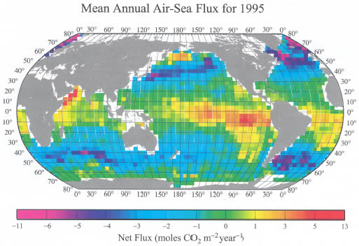
Figure 6. Distribution of the climatological mean annual sea-air CO![]() flux
(moles CO
flux
(moles CO![]() m
m![]() yr
yr![]() )
for the reference year 1995 representing non-El Niño conditions. This
has been computed using the mean monthly distribution of sea-air pCO
)
for the reference year 1995 representing non-El Niño conditions. This
has been computed using the mean monthly distribution of sea-air pCO![]() difference,
the climatological NCEP 41-year mean wind speed and the wind-speed dependence
of the CO
difference,
the climatological NCEP 41-year mean wind speed and the wind-speed dependence
of the CO![]() gas
transfer velocity of Wanninkhof
(1992). The yellow-red colors indicate a region characterized by a net
release of CO
gas
transfer velocity of Wanninkhof
(1992). The yellow-red colors indicate a region characterized by a net
release of CO![]() to
the atmosphere, and the blue-purple colors indicate a region with a net uptake
of CO
to
the atmosphere, and the blue-purple colors indicate a region with a net uptake
of CO![]() from
the atmosphere. This map yields an annual oceanic uptake flux for CO
from
the atmosphere. This map yields an annual oceanic uptake flux for CO![]() of
2.2 ± 0.4 Pg C yr
of
2.2 ± 0.4 Pg C yr![]() .
.
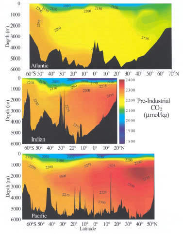
Figure 7. Zonal mean pre-industrial distributions of dissolved inorganic
carbon (in units of µmol kg![]() )
along north-south transects in the Atlantic, Indian and Pacific oceans. The
Pacific and Indian Ocean data are from the Global CO
)
along north-south transects in the Atlantic, Indian and Pacific oceans. The
Pacific and Indian Ocean data are from the Global CO![]() Survey
(this study), and the Atlantic Ocean data are from Gruber
(1998).
Survey
(this study), and the Atlantic Ocean data are from Gruber
(1998).
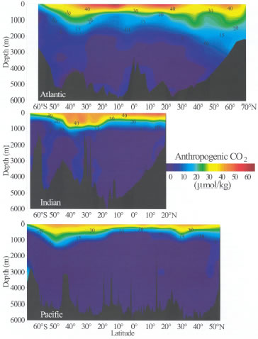
Figure 8. Zonal mean distributions of estimated anthropogenic CO![]() concentrations
(in units of µmol kg
concentrations
(in units of µmol kg![]() )
along north-south transects in the Atlantic, Indian and Pacific oceans. The
Pacific and Indian Ocean data are from the Global CO
)
along north-south transects in the Atlantic, Indian and Pacific oceans. The
Pacific and Indian Ocean data are from the Global CO![]() Survey
(this study), and the Atlantic Ocean data are from Gruber
(1998).
Survey
(this study), and the Atlantic Ocean data are from Gruber
(1998).
Figure 9. Zonal mean anthropogenic CO![]() inventories
(in units of moles m
inventories
(in units of moles m![]() )
in the Atlantic, Indian and Pacific oceans.
)
in the Atlantic, Indian and Pacific oceans.
Return to previous section or return to Abstract