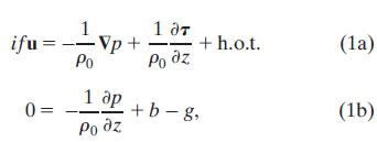
We will consider the most basic framework for interpreting near-surface currents at 2°N: the linear, steady-state equations of motion in hydrostatic balance:
where i is ![]() , u is the horizontal velocity vector, f is the vertical component of the Coriolis parameter, ρ0 is the background density, ∇ is the horizontal gradient operator, p is pressure, g is gravity, and b = g(ρ0 − ρ)/ρ0 is buoyancy. Here h.o.t. refers to higher-order terms (e.g., horizontal eddy stress terms), which, for simplicity, we assume to be negligible. We then make the standard assumptions that the stress vector within the fluid, τ(z), can be related to the shear profile through a turbulent viscosity parameter ν,
, u is the horizontal velocity vector, f is the vertical component of the Coriolis parameter, ρ0 is the background density, ∇ is the horizontal gradient operator, p is pressure, g is gravity, and b = g(ρ0 − ρ)/ρ0 is buoyancy. Here h.o.t. refers to higher-order terms (e.g., horizontal eddy stress terms), which, for simplicity, we assume to be negligible. We then make the standard assumptions that the stress vector within the fluid, τ(z), can be related to the shear profile through a turbulent viscosity parameter ν,
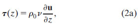
and that, at the surface, the shear stress balances the wind stress, τ0:
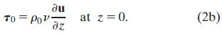
The bottom boundary condition for (1) is less straight-forward, as will be discussed.
At depths where both ν = 0 and ∂ν/∂z = 0, the flow is inviscid and (1a) reduces to the geostrophic balance. Because depth variations in the pressure gradient can be related to the buoyancy gradient by (1b), the geostrophic shear is parallel to density contours and is referred to as "thermal wind shear":
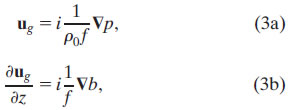
where ug is the geostrophic velocity. Near 2°N in the eastern and central Pacific, a strong temperature front exists between the cold water upwelled at the equator and the warm water advected east by the North Equatorial Counter Current. We therefore expect strong thermal wind shear oriented along this front.
Away from the equator and in regions with no fronts, that is, where the shear is entirely ageostrophic, the stress divergence effects can be separated from the pressure gradient by decomposing the velocity in (1a) into geostrophic and ageostrophic components (u = ug + ua ). Following Ekman (1905), Eq. (1a) can be further simplified by assuming that viscosity is vertically uniform. Invoking the standard top boundary condition that surface shear is proportional to the wind stress (2b) and making a no-drag bottom boundary condition, the "classical Ekman" model for the ageostrophic velocity profile then becomes
classical Ekman: 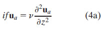
with boundary conditions:
where H is some depth below the frictional layer, functionally set as ∞.
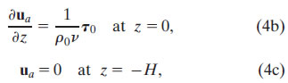
We now consider the Ekman response in frontal regions. Above the top of the thermocline (roughly 125 m at 2°N, 140°W), vertical mixing likely causes the subsurface frontal structure to be similar to the surface. Within the thermocline, though, the horizontal temperature gradient probably differs from the sea surface temperature (SST) gradient. For simplicity and because we lack more detailed information, we will assume that the buoyancy front within the upper ocean is vertically uniform and equivalent to the surface front. By (3b), this implies that the geostrophic shear is also vertically uniform and therefore does not enter the stress divergence term on the rhs of (1a). Equation (1a) thus reduces to
Ekman uniform front:
which is identical to the classical Ekman model (4a). The vertically uniform geostrophic shear, however, will contribute to the top boundary condition (2b), which can be rearranged to be a boundary condition for the ageostrophic profile:
where, as in (4), viscosity is assumed to be vertically uniform. The bottom boundary condition (5c) states that the influence of the wind dies out by z = −H, and at that level the flow is geostrophic. Note that the "frontal Ekman" model (5) resembles the classical Ekman model (4), with the important distinction that the effective surface stress τeff that forces the ageostrophic Ekman spiral is only a portion of the wind stress—the portion that is out of balance with the surface geostrophic shear stress
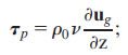
that is, τeff = τ0 − τp. In other words, in a region with a vertically uniform front, the ageostrophic Ekman spiral is a linear sum of the classic response to the wind stress τ0 and a second spiral forced by −τp. This second ageostrophic spiral counterbalances the surface geostrophic shear associated with the front, assuring that the total surface shear satisfies the boundary condition (2b).
Because the geostrophic shear depends on the factor 1/f, the stress contribution from a given surface density gradient is larger in tropical regions than at higher latitudes. At the equator, however, geostrophic shear is undefined. As shown by Stommel (1960), on the equator, the zonal wind stress tends to balance the zonal pressure gradient. Assuming steady, linear, homogenous flow, with uniform viscosity, Stommel determined an analytic solution for p and u that satisfied
Stommel model: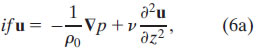
with boundary conditions:
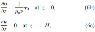
in addition to eastern and western boundary conditions on the zonal transport. Unlike the Ekman "no-drag" bottom boundary condition, the Stommel bottom boundary condition (6c) requires that the shear (and thus stress) is zero at the fixed level z = − H, nominally set as the center of the Equatorial Undercurrent (EUC). The resulting solution is valid both on and off the equator and reproduces many of the features of the equatorial current system including a South Equatorial Current lying above an EUC.
Fronts, however, are a ubiquitous feature of the global oceans, and the assumption in the original Stommel model that density gradients are negligible is one of its major limitations. The Stommel model was extended to include fronts by Schneider and Müller (1994), and Bonjean and Lagerloef (2002, hereafter referred to as BL02) derived an analytical solution for the vertical shear in the extended Stommel model. Both derivations assume vertically uniform fronts and vertically uniform viscosity. In particular, the analytical solution for the shear enabled BL02 to determine the effects of mixing at 30 m on the upper 30-m layer currents (which are given a nominal depth of 15 m). To map the global 15-m currents, BL02 estimate viscosity from wind speed based upon the Santiago-Mandujano and Firing (1990) empirical relationship, determine the buoyancy gradient from the Tropical Rainfall Measuring Mission (TRMM) Microwave Imager (TMI) SST, and the surface pressure gradient and wind stress from satellite altimetry and scatterometer fields. The resulting 15-m velocity product is referred to as the Ocean Surface Current Analyses—Real time (OSCAR) and is available online at www.oscar.noaa.gov).
While the boundary conditions (6b)–(6c) invoked by Stommel (1960) have become widely used, they are not always realistic. Stommel notes that, while the zero shear bottom boundary condition (6c) is satisfied at the center of the EUC, the EUC shoals to the east and therefore the no-stress level is not strictly flat. Likewise, poleward of the EUC, the shear is not generally zero at this depth (e.g., the thicker South Equatorial Currents flank the EUC). This is particularly a problem for the BL02 formulation that assumes vertically uniform fronts and thus vertically uniform geostrophic shears (3b). In this case, the zero total shear bottom boundary condition (6c) implicitly requires an ageostrophic shear at z = −H that is equal and opposite to the thermal wind component. BL02 argued that the shear solution at 30 m is relatively insensitive to H and chose H based upon a best-fit procedure to be 70 m for the OSCAR product. In contrast, the Ekman frontal model (5) allows the flow to transition to geostrophic flow at H, but has a singularity at the equator.
The conundrum can be resolved if the viscosity decays with depth so that, at the base of the frictional layer, the stress becomes zero, while the shear can remain nonzero. This assumption is consistent with microstructure measurements (e.g., Peters et al. 1988; Smyth et al. 1996) that show a several decade reduction in viscosity between the surface mixed layer and deeper thermocline values. An equation for the stress can then be derived by taking the vertical derivative of (1) and expressing shear in terms of the stress (2a):
generalized Ekman: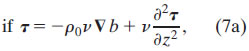
As in the classical Ekman model (4) and frontal Ekman model (5), viscosity and buoyancy gradient profiles are prescribed. The buoyancy gradient in (7a), however, is not required to be vertically uniform, so this "generalized Ekman" model (7) is valid for regions in which the front is tilted. Furthermore, because f does not appear in the denominator of (7), the generalized Ekman model is also valid both on and off the equator. With viscosity and buoyancy gradient profiles known or assumed, (7) can be solved numerically for τ, and the stress–shear relationship (2a) can then be used to determine the shear flow profile. The shear can then be decomposed into geostrophic and ageostrophic components according to (3b).
Finally, it is worth considering the effect of these assumptions on the geostrophic and ageostrophic (Ekman) transport. By vertically integrating (1a) from the surface to the depth −H, the transport U can be expressed as
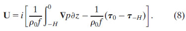
The first term on the rhs of (8) is the geostrophic transport; the last two terms are the ageostrophic Ekman transport associated with the surface wind stress (τ0) and with the stress at the base of the frictional layer (τ−H). A front modifies the total transport in the direction of the front through the geostrophic term and potentially modifies the transport perpendicular to the front through the Ekman transport associated with τ−H. In particular, if, as in the case of the frontal Ekman model (5), the viscosity is not zero at the depth −H and a thermal wind shear exists at that depth, then τ−H will be nonzero and will induce an ageostrophic Ekman transport in the direction of the density gradient, that is, perpendicular to the front. However, if viscosity tapers to zero at depth −H, as in the generalized Ekman model (7), then the net Ekman transport is to the right of the wind and invariant to the front. The Ekman transport in the generalized Ekman model is thus identical to that in the classical Ekman model (4) and differs from the frontal Ekman model transport. Since the generalized and frontal Ekman models differ primarily in their bottom boundary conditions, it is likely that their differences are most apparent in the lower portion of their Ekman spirals.
The remainder of this paper will explore the consequences of the two principal mechanisms by which a vertically uniform front affects the near-surface currents: First, through the surface boundary condition (2b), in which the geostrophic shear contributes to the total surface shear ∂u/∂z, thereby modifying the effective stress that forces the ageostrophic flow, and second, through the front's geostrophic interior shear that is added to the ageostrophic Ekman spiral. If the front is tilted, then additional possibilities arise, which cannot be evaluated from the single mooring studied here. Nevertheless, as we will show, even a simple vertically uniform front produces systematic changes in the magnitude and direction of the near-surface currents. In the region of the cold tongue front, near-surface flow lies within the poleward branch of the tropical Pacific meridional overturning cell. The consequences of the front, therefore, can include modifying the large-scale overturning circulation.
Return to Previous section
Go to Next section