 + 1000) according to the UNESCO 1983 polynomial [Fofonoff
and Millard, 1983]. Figures 3-4
show the surface and subsurface time series at 0°, 156°E during the 3-month
deployment.
+ 1000) according to the UNESCO 1983 polynomial [Fofonoff
and Millard, 1983]. Figures 3-4
show the surface and subsurface time series at 0°, 156°E during the 3-month
deployment. The upper ocean heat budget in the western equatorial Pacific warm pool is analyzed for a 3-month period from mid-September through mid-December 1992 using data from the Tropical Atmosphere Ocean (TAO) array enhanced for the Coupled Ocean Atmosphere Response Experiment. Surface heat and moisture fluxes were measured from a centrally located TAO current meter mooring at 0°, 156°E. Lateral heat advection was estimated using temperature data from moorings within 150-250 km of 0°, 156°E. Mixing was estimated as the residual of the heat balance and compared to estimates of mixing based on the Niiler-Kraus parameterization of entrainment mixing. The analysis shows that for the diurnal cycle and for daily to weekly timescale variations like those associated with westerly wind bursts, the sea surface temperature (SST) variability is to a large extent controlled by shortwave radiation and latent heat flux. However, three-dimensional processes can also be important. For example, in early October 1992, the SST at 0°, 156°E increased by nearly 1°C in 7 days due predominately to westward heat advection. Also, the dynamical response to a moderately strong wind burst in late October 1992 included a deepening of the pycnocline, which affected the rate of entrainment cooling, and a reversal of the surface current, which affected the zonal heat advection. The importance of three-dimensional processes (particularly heat advection) in the warm-pool heat balance during this 3-month study period is confirmed by comparing the observed temperature variability with that simulated by a one-dimensional mixed layer model.
The western equatorial Pacific is characterized by mean sea surface temperatures (SSTs) in excess of 28°C, weak trade winds, and deep atmospheric convection [Bjerknes, 1969; Graham and Barnett, 1987]. While the western equatorial Pacific "warm pool" SST is relatively homogenous in comparison to other regions of the world's oceans, small O(1°C) variations in the magnitude of the SST can result in dramatic shifts in global weather patterns [Palmer and Mansfield, 1984]. Understanding the processes controlling warm pool SST variability is thus vital for understanding the global climate variability.
For timescales longer than a day, variability in the surface forcing is associated primarily with westerly wind bursts that last several days to weeks. Climatically, these westerly wind bursts tend to occur more frequently during the November-April months of a developing El Nińo and result in a slackening of the trades [Barnett, 1977; Luther et al., 1983; Harrison and Giese, 1991]. Intensified wind speeds and cloudiness associated with the wind bursts contribute to surface cooling due to enhanced latent heat loss and reduced shortwave radiation [Meyers et al., 1986; McPhaden and Hayes, 1991; Zhang and McPhaden, 1995; Zhang, 1996]. Increased eastward wind stress during a westerly wind burst can also cause the surface current to accelerate eastward, and the pycnocline to deepen due to both turbulent mixing and Ekman convergence [McPhaden et al., 1988, 1992]. Additionally, heavy rainfall associated with a wind burst may produce a shallow freshwater stratified barrier layer which can inhibit vertical turbulent heat fluxes [Godfrey and Lindstrom, 1989; Lukas and Lindstrom, 1991; Sprintall and McPhaden, 1994; Anderson et al., 1996]. Thus westerly wind bursts can affect all terms in the heat balance: radiative and turbulent surface heat fluxes, turbulent mixing, and advection, with potentially significant impacts on the evolution of longer-period climate variability. Moreover, wind bursts can trigger equatorial Kelvin waves that propagate into the central and eastern equatorial Pacific, where they may lead to SST warming and possible additional climate feedbacks [Miller et al., 1988; Kessler et al., 1995].
A major goal of the Tropical Ocean Global Atmosphere-Coupled Ocean Atmosphere Response Experiment (TOGA-COARE) was to describe and understand the principal processes responsible for the coupling of the ocean and atmosphere in the western Pacific warm pool system. The intensive observation period (IOP) (November 1992 through February 1993) was chosen because wind bursts have a higher frequency of occurrence during these months. Oceanic and meteorological field work in the warm pool was predominately concentrated within the 150 km × 150 km Intensive Flux Array (IFA) centered at 2°S, 156°E. The IFA was imbedded within a larger array of Tropical Atmosphere and Ocean (TAO) moored buoys [McPhaden, 1993b] enhanced with additional moorings and instrumentation specifically for COARE [Webster and Lukas, 1992].
In the analysis presented here, the upper ocean heat balance is evaluated using enhanced instrumentation on a TAO buoy at 0°, 156°E. The buoy's deployment period (September 15 through December 20, 1992) spans the October 1992 westerly wind burst which peaked just as the COARE IOP was commencing. As discussed in section 4, the ocean response to this moderate westerly wind burst was dramatic and included a cooling of the SST by nearly 1°C, a deepening of the pycnocline by 50 m, and a reversal of the surface currents.
The data used in this analysis are described in the following section. In section 3, the details of the heat balance analysis are described. In section 4, the surface conditions, subsurface conditions, and the resulting variability in the heat balance are described. An important finding of the analysis is that heat advection can at times be the dominant mechanism controlling warm pool SST variability. In section 5, the heat flux due to entrainment mixing is estimated from the turbulent energy equation following Niiler and Kraus [1977] and compared to the residual of the observed heat balance. Section 6 investigates the importance of three-dimensional processes by comparing the observations to the variability simulated with the Price et al. [1986] one-dimensional mixed layer model. The final two sections discuss and summarize the key results of the paper.
Figure 1 shows the TOGA-COARE enhanced monitoring
array of TAO buoys. The data in this analysis derive primarily from a PROTEUS
(PROfile TElemetry of Upper ocean currentS) buoy which was deployed at 0°0.1'S,
156°2.3'E on September 15, 1992. On December 20, 1992, the buoy broke away from
its anchor, but within several days the buoy and subsurface mooring instrumentation
were successfully recovered. By comparing data from the mechanical current meters
and the downward-looking acoustic Doppler current profiler (ADCP) attached to
the buoy's bridle, it was determined that the mooring line had become entangled
with itself on deployment such that instruments below 50 m were shifted up 18
m. A schematic of the 0°, 156°E PROTEUS buoy with the depth-shifted instrumentation
is shown in Figure 2. Table 1 lists the depths
and duration of the subsurface temperature, salinity, and current velocity instrumentation.
As shown in Figure 2 and Table 2, surface data
from the buoy include vector winds, air temperature, relative humidity, rain
rate, and shortwave radiation. SST and sea surface salinity were measured at
1 m depth. All surface and subsurface PROTEUS data were averaged hourly and
subsampled once per hour centered on the half hour. Collocated temperature and
salinity were used to estimate potential density (
+ 1000) according to the UNESCO 1983 polynomial [Fofonoff
and Millard, 1983]. Figures 3-4
show the surface and subsurface time series at 0°, 156°E during the 3-month
deployment.
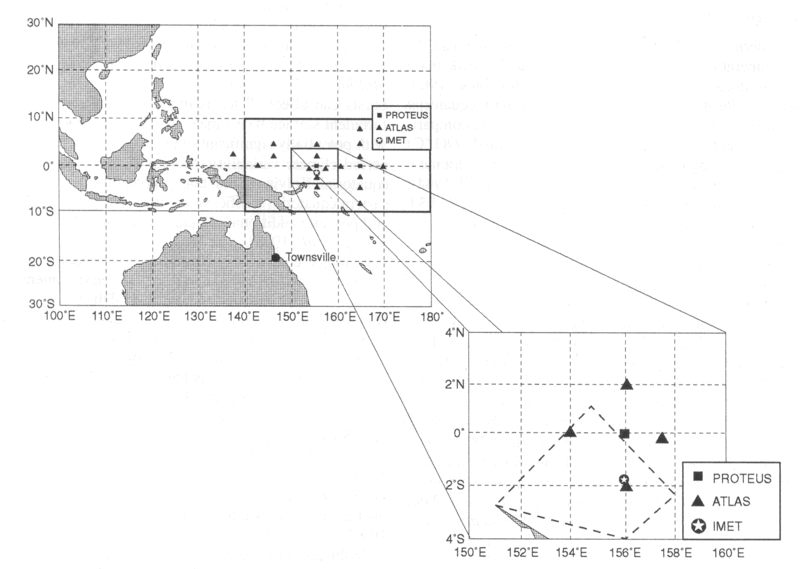
Figure 1. The enhanced monitoring array. The heat balance is estimated at the central 0°, 156°E PROTEUS mooring. The four nearest ATLAS buoys at 0°, 154°E; 0°, 157.5°E; 2°N, 156°E; and 2°S, 156°E are used to estimate horizontal temperature gradients. The 0°, 156°E PROTEUS mooring is on the northern edge of the COARE intensive flux array (dashed region).
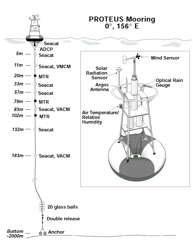
Figure 2. Diagram of the PROTEUS buoy which was deployed at 0°, 156°E from September 15 to December 20, 1992. The vector averaging current meters (VACMs) are located 1 m above the listed SEACAT depths.
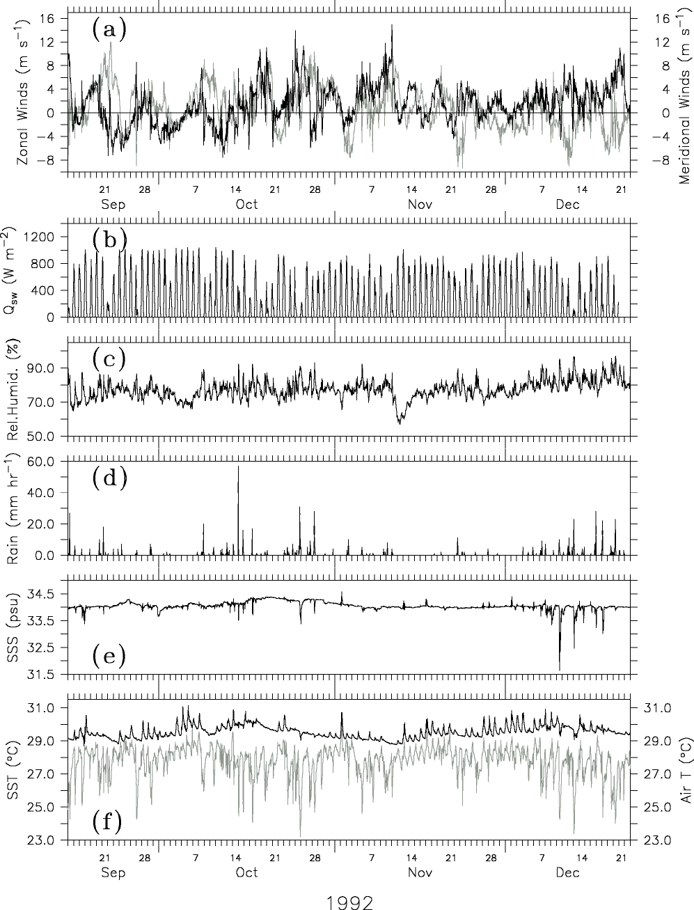
Figure 3. Hourly surface data: (a) eastward (dark line) and northward (light line) winds, (b) shortwave radiation, (c) relative humidity, (d) rain, (e) 1-m sea surface salinity (SSS), and (f) air temperature (light line) and 1-m sea surface temperature (SST) (dark line).
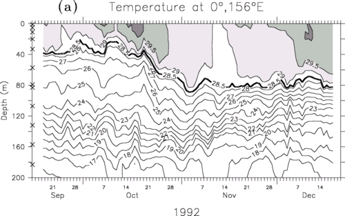
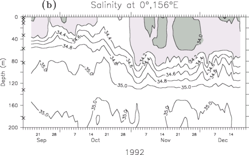
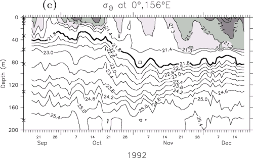
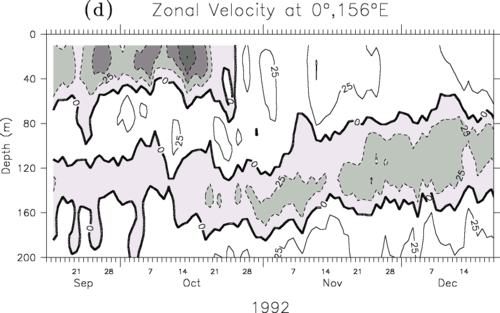
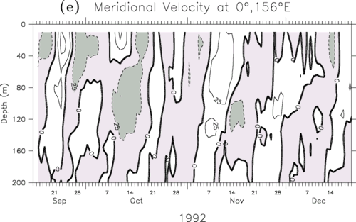
Figure 4. Daily averaged subsurface (a) temperature, (b) salinity,
(c) potential density, (d) ADCP zonal flow, and (e) meridional flow. The surface
layer is defined as the depth of the 21.8 kg m density surface (ATLAS moorings use the 28.5°C isotherm as the surface layer
depth). The subsurface temperature contour interval (CI) is 1°C for values less
than 28°C and 0.5°C for warmer values. The salinity CI is 0.2 psu. The density
CI is 0.1 kg m for values less than 21.4
kg m and 0.4 kg m
for denser values. The velocity CI is 25 cm s
density surface (ATLAS moorings use the 28.5°C isotherm as the surface layer
depth). The subsurface temperature contour interval (CI) is 1°C for values less
than 28°C and 0.5°C for warmer values. The salinity CI is 0.2 psu. The density
CI is 0.1 kg m for values less than 21.4
kg m and 0.4 kg m
for denser values. The velocity CI is 25 cm s .
Westward and southward directed currents are contoured with dashes.
.
Westward and southward directed currents are contoured with dashes.
Table 1. Subsurface PROTEUS Instrumentation Used in This Analysis
| Depth | Instrument | Variable | Record start and end dates |
| bridal | ACDP | u, v | Sept. 15 to Dec. 24, 1992 |
| 1 | SEACAT | T, S | Sept. 15 to Dec. 24, 1992 |
| 5 | SEACAT | T, S | Sept. 15 to Dec. 24, 1992 |
| 10 | VAC | u, v | Sept. 15 to Dec. 24, 1992 |
| 11 | SEACAT | T, S | Sept. 15 to Dec. 24, 1992 |
| 20 | MTR | T | Nov. 5 to Dec. 13, 1992 |
| 33 | SEACAT | T, S | Sept. 15 to Dec. 20, 1992 |
| 57 | SEACAT | T, S | Sept. 15 to Dec. 20, 1992 |
| 79 | MTR | T | Nov. 5 to Dec. 13, 1992 |
| 82 | VACM | u, v | Sept. 15 to Dec. 20, 1992 |
| 83 | SEACAT | T, S | Sept. 15 to Dec. 20, 1992 |
| 107 | MTR | T | Sept. 15 to Dec. 20, 1992 |
| 132 | SEACAT | T, S | Sept. 15 to Dec. 20, 1992 |
| 182 | VACM | u, v | Sept. 15 to Dec. 20, 1992 |
| Depths represent best estimates of actual depth. Variables measured include temperature (T), salinity (S), and zonal (u) and meridional (v) velocity. | |||
As shown in Table 1, subsurface temperatures on the 0°, 156°E PROTEUS mooring were measured with mini-temperature recorders (MTR) designed and manufactured at the NOAA Pacific Marine Environmental Laboratory, and with Seabird Electronics, Inc. SEACATS. In order to estimate the horizontal temperature gradients, daily averaged subsurface temperature data were used from nearby ATLAS moorings at 0°, 154°E; 0°, 157.5°E; 2°N, 156°E; and 2°S, 156°E, shown in Figure 1. ATLAS moorings have 11 thermistors located at depths of 1, 25, 50, 75, 100, 125, 150, 200, 250, 300, and 500 m. On the basis of laboratory predeployment and postdeployment calibrations [McCarty and McPhaden, 1993; Freitag et al., 1994], SST accuracy is 0.01°C for the PROTEUS mooring and 0.03°C for ATLAS moorings; subsurface temperature accuracy is 0.01°C for the PROTEUS mooring and 0.09°C for ATLAS moorings.
SEACATs were also used to measure subsurface salinity on the 0°, 156°E PROTEUS mooring. Precalibrations and post-calibrations showed drifts in some SEACAT conductivity sensors equivalent to a salinity drift of up to -0.03 psu in 4 months. By using a linear weighted average of the precalibration and postcalibration coefficients, nearly all density inversions within the mixed layer were eliminated, and an in-situ comparison with 90 CTDs taken within 5 km of the mooring by the R/V Hakuho-Maru during November 10-25, 1992, was significantly improved.
An RD Instruments, downward-looking 153.6-kHz ADCP measured current velocity
from 14 m to approximately 250 m in 8-m bins. At 10 m depth, current velocities
were measured by a EG&G model 610 vector averaging current meter (VACM).
For purposes of the analysis it was assumed that velocities shallower than 10
m had no shear. The 82- and 182-m VACMs were used only to determine the depth
correction as discussed earlier. The errors in current speed and direction were
assumed to be 3 cm s and 2°, respectively
[Lien
et al., 1994; P. Plimpton, personal communication, 1996].
Vector winds at 0°, 156°E were measured with a RM Young wind sensor and vane
located 4 m above the ocean surface atop the buoy tower. As listed in Table
2, the sensor's resolution is 0.2 m s. Air
temperature and relative humidity were measured 3 m above the surface by a Rotronic
Instrument Corporation model MP-100 temperature-humidity probe with shielding
to reduce the effects of radiative heating. The sensors, however, were unaspirated,
so errors may be larger when winds are light on sunny days. No postcalibrations
were obtained for the thermistor and relative humidity sensor because the thermistor
failed during postcalibration procedure. However, in-situ comparisons with the
R/Vs Le Noroit, Hakuho-Maru, Natsushima, and Moana Wave
when these ships were within 3-15 km of the buoy suggest that the buoy's relative
humidity measurements were 3% too low at deployment and had a linear drift of
0.9% month. Freitag
et al. [1994] show that individual humidity sensors of this generation
could have offsets and drifts of similar magnitude. Thus the relative humidity
data have been adjusted to agree with the ship measurements. This correction
to the relative humidity results in a more consistent heat balance, described
in section 4.
Table 2. Standard Deviations of the 5-Day Triangular Filtered Surface Measurements, Typical Measurement Errors, and Resulting Errors in Bulk Fluxes
| Instrument |
Variable |
5-Day Filtered Std Dev |
Typical Error |
Corresponding rms Error, W
m |
|||
Q |
Q |
Qrf | Q |
||||
| RM Young | winds | 1.41 m s |
0.20 m s |
4.7 | 0.5 | 0.1 | 5.1 |
| Rotronics | air temperature | 0.38°C | 0.16°C | 0.6 | 1.3 | 0.2 | 1.8 |
| Rotronics | relative humidity | 0.03 | 0.02 | 9.2 | 0.1 | 0.6 | 9.2 |
| SEACAT | SST | 0.30°C | 0.014°C | 0.4 | 0.1 | 0.0 | 0.5 |
| ORG | rain rate | 0.37 mm h |
25% | 0.0 | 0.0 | 2.9 | 2.9 |
| Eppley | Qsw | 40 W m |
2-3.5% | 0.2-0.3 | 0.1 | 0.0 | 6.4-11.3 |
| The 2% error in the shortwave radiation, Qsw, is the standard error assuming the radiometer mast is vertical. This error increases to a maximum of 3.5% if the mast is tilted 15° from the vertical. To estimate the upper and lower limits of the resulting flux errors, the bulk heat flux algorithm was run with the observed variables with plus and minus typical errors. One half the rms difference between the upper and lower limit is listed as the corresponding rms error in the heat flux due to a typical error in the bulk parameter. | |||||||
Hourly rain rates were measured by a Science Technology, Inc. model 105 optical rain gauge (ORG). The instrument computes a rain rate proportional to scintillations caused by rain drops falling through a beam of near-infrared light [Wang and Crosby, 1993]. A description of the ORG mounting, sampling, and signal-processing characteristics for application on TAO buoys is given by McPhaden and Milburn [1992]. The accuracy of moored ORG measurements has been difficult to determine for lack of sufficient calibration data in natural rain rates prior to the COARE field phase (the particular instrument used in this study was nonfunctional on return and could not be postcalibrated). Most potential error sources (e.g., vibration, drop-size dependence, and splash from the instrument housing) would lead to relative uncertainties of O(10%) [e.g., McPhaden, 1993a; Thiele et al., 1994; F. Bradley, personal communication, 1996]. Probably the greatest uncertainty is simply in the factory calibrations which, if used without further correction, can lead to differences between like instruments of 15-30% [Thiele et al., 1994]. For our purposes we assume an error of 25%.
Shortwave radiation was measured by an Epply radiometer with a calibration
accuracy of 2%. Although the radiometer has a full record up to when the buoy
broke away from its anchor, the radiometer and its mast were missing when the
buoy was recovered. Photos taken from the R/V Hakuho-Maru on November
20, 1992, show that the radiometer mast had been bent and was tilted at about
15° from the vertical. The buoy had apparently been vandalized. Although it
is not clear when the vandalism occurred, the fact that the November 13 noontime
radiation exceeded 1000 W m suggests that
the buoy had been vandalized sometime after November 13. The tilt could produce
an error as large as 3%; however, on overcast days on which the radiation is
diffuse, the error produced by the tilt should be negligible. We have therefore
made no attempt to correct for this error. Instead, we assume that the shortwave
radiation error is 2% prior to November 20 and thereafter is 3.5%.
The surface heat flux is estimated as
| (1) |
where  is the albedo, Qsw
is the incoming shortwave radiation, Qlw is the net longwave
radiation, Q is the latent
heat flux, Q is the sensible
heat flux of the cool air over the warm water, and Qrf is
the sensible heat flux due to rain.
is the albedo, Qsw
is the incoming shortwave radiation, Qlw is the net longwave
radiation, Q is the latent
heat flux, Q is the sensible
heat flux of the cool air over the warm water, and Qrf is
the sensible heat flux due to rain.
As described earlier, the shortwave radiation, Qsw, was measured by an Epply radiometer. A constant albedo value of 0.055 is used based on measurements taken aboard the R/V Franklin [P. Coppin and F. Bradley, personal communication, 1994]. Net longwave radiation, Qlw, is estimated using the Clark et al. [1974] bulk formula [Fung et al., 1984]:
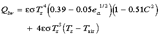 |
where  = 0.97 is the emissivity,
  = 5.67 × 10
 W m
K
W m
K is the Stephan Boltzmann constant, T
 is the near-surface air temperature (in kelvins), e
 is the near-surface vapor pressure (in millibars), Ts is the
1-m-depth sea surface temperature (in kelvins), and C is the cloud cover
index which ranges from 0 (clear sky) to 1 (cloud-covered sky). C is
estimated by inverting Reed's
[1977] expression for the daily averaged insolation Qsw:
is the near-surface vapor pressure (in millibars), Ts is the
1-m-depth sea surface temperature (in kelvins), and C is the cloud cover
index which ranges from 0 (clear sky) to 1 (cloud-covered sky). C is
estimated by inverting Reed's
[1977] expression for the daily averaged insolation Qsw:
where Qcs is the clear-sky radiation and n is the
noontime solar altitude. These daily estimates of C are then interpolated
to hourly values to estimate hourly net longwave radiation. Intercomparison
with the shipboard measurements of incoming longwave radiation suggests that
the root mean square (rms) error in Qlw is 6 W m.
Latent and sensible heat loss rates are estimated using the COARE version 2.5
bulk formulae [Fairall
et al., 1996a], which are based on Liu
et al. [1979]. The algorithm includes a cool skin parameterization
and a simplified Price
et al. [1986] mixed layer model to extrapolate bulk SST measurements
to the interface z = 0 [Fairall
et al., 1996b]. Additionally, the wind speeds are measured relative
to the sea surface velocity (assumed here to be identical to the velocity at
10 m depth), and a gustiness factor which depends upon the convective scaling
velocity is included for low wind conditions. The COARE bulk algorithm also
estimates the sensible heat flux due to rain Qrf by assuming
that the rain falls at the wet-bulb temperature. Time series of the heat fluxes
are shown in Figure 5. Figure
6 shows the time series of the net surface heat flux, Q.
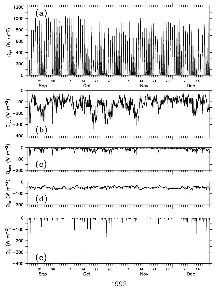
Figure 5. Hourly air-sea heat fluxes. (a) Shortwave radiation, Qsw,
(b) latent heat flux, Q,
(c) sensible heat flux, Q,
(d) net longwave radiation, Qlw, and (e) sensible heat flux
due to rain, Qrf .
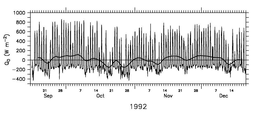
Figure 6. Hourly and 5-day triangular filtered net surface heat flux. A positive flux value represents a heat flux into the ocean.
To estimate rms errors in the turbulent heat fluxes due to typical errors in
the bulk variables (wind speed, air temperature, relative humidity, SST, rain,
and shortwave radiation), the flux algorithm was run sequentially with observed
values ±1 standard error (i.e., twelve runs for the six bulk variables). The
errors listed in Table 2 were then computed as one-half the rms difference between
the flux time series estimated with values +1 standard error and -1 standard
error of the corresponding input variable. Errors due to inadequate parameterization
of the turbulent fluxes are not included, so our error estimates for bulk fluxes
should be considered as lower bounds. Latent heat flux is sensitive primarily
to errors in relative humidity and to a lesser extent to errors in wind speed
(Table 2), and the resulting latent heat flux error is similar in magnitude
to the rms error in the shortwave radiation (Table 3). Errors in shortwave radiation,
air temperature, and SST have a relatively small effect on the turbulent heat
fluxes. The record length mean net surface heat flux is not significantly different
than zero. However, since the standard deviation of the 5-day filtered net surface
heat flux is more than 4 times larger than the rms error, the data can resolve
the variability in the surface heat fluxes on wind burst timescales which are
highlighted by the 5-day triangular filter (cutoff frequency = (3 - day),
half amplitude frequency = (6.77 - day)).
| Table 3. Record Length Means, Standard Deviations of the 5-Day Triangular Filtered Fluxes, rms Error, and Cross Correlations Between 5-Day Filtered Fluxes and 5-Day Filtered Wind Speed | ||||
| Heat Flux | Mean, W m |
5-Day Filtered Std Dev, W m |
rms Error, W m |
5-Day Filtered Correlation with Wind Speed |
| (1-)Qsw |
189 | 38 | 6.6-11.5 | -0.57 |
| Qlw | -48 | 5 | 6 | 0.70 |
| Q |
-118 | 34 | 10.3 | -0.93 |
| Q |
-11 | 5 | 1.4 | -0.69 |
| Qrf | -2 | 2 | 3.0 | -0.32 |
| Q |
10 | 68 | 14.2-16.9 | -0.80 |
Following Stevenson and Niiler [1983], the vertically averaged heat balance within the surface layer can be expressed as a tendency balance:
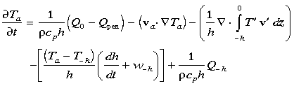 |
(2a) |
or alternatively as a heat flux balance:
 |
(2b) |
where  cp is the volumetric
heat capacity of seawater, taken to be 4.088 × 10
cp is the volumetric
heat capacity of seawater, taken to be 4.088 × 10 J °C-1 m; Ta
and va are the vertically averaged temperature and
horizontal velocity within the layer; T
J °C-1 m; Ta
and va are the vertically averaged temperature and
horizontal velocity within the layer; T and v are the deviations from the vertical
averages
and v are the deviations from the vertical
averages
 |
T-h and w-h are the temperature and vertical
velocity at the layer depth z = -h; Q
is the net radiative and turbulent surface heat flux as described in section
2.2; Q is the amount of
shortwave radiation that penetrates through the base of the layer z =
-h; and Q-h is the turbulent diffusion at the base
of the layer.
is the amount of
shortwave radiation that penetrates through the base of the layer z =
-h; and Q-h is the turbulent diffusion at the base
of the layer.
In this analysis we define the surface layer as the weakly stratified portion
of the water column from the ocean surface to the isopycnal 21.8 kg m,
i.e., -h = z( = 21.8
kg m). The analysis was essentially unchanged
when a deeper isopycnal (22.2 kg m) was
used. Note that if this isopycnal is a material surface, then w-h
= -dh/dt and thus vertical entrainment (terms in (2) involving
dh/dt + w-h) would be identically equal
to zero. As can be seen in the density profile time series (Figure
4c), the 21.8 kg m isopycnal is near
the top of the pycnocline. During the first month of the record the surface
layer according to this definition was on average only 35 m deep and at times
as shallow as 17 m. We can therefore expect entrainment across this layer depth
to be nonzero, which is in fact borne out in the calculations described in section
5.
This surface layer, with its bottom boundary defined by the 21.8 kg m
isopycnal surface, is distinct from the diurnal mixed layer. During periods
of light wind, the daytime diurnal mixed layer depth can be within several meters
of the surface and thus cannot be properly resolved with the mooring data, while
during nighttime, entrainment mixing causes the diurnal mixed layer to approach
the top of the pycnocline (i.e., the surface layer depth). Although the vertically
averaged temperature of the weakly stratified surface layer Ta
is not necessarily identical to SST, as shown in Figure
7, Ta tends to track the lower-frequency variability in
SST, while filtering out the diurnal variability. Thus the surface layer heat
balance can be used to identify processes responsible for variability in the
SST on wind burst timescales.
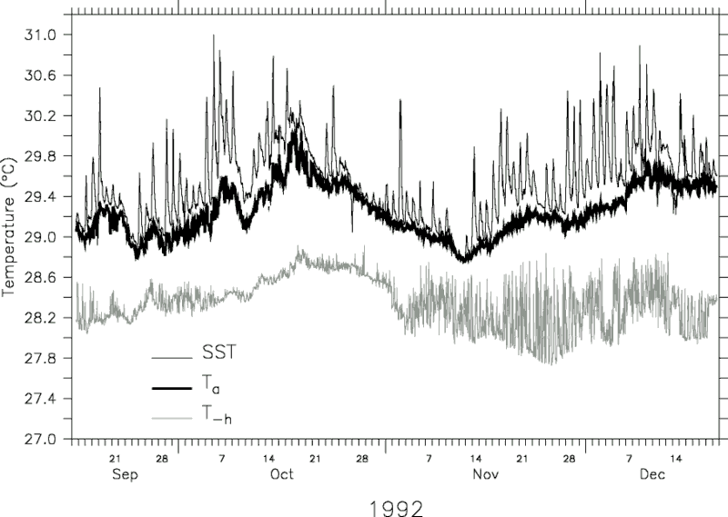
Figure 7. Hourly time series of the vertically averaged surface layer
temperature (Ta), SST at 1 m depth, and the temperature at
the base of the surface layer (Th, where the base of the surface
layer is defined as the depth of the 21.8 kg m
density surface).
Comparisons with 90 conductivity-temperature-depth profiles (CTDs) (with vertical
resolution of 1 m) indicate that the rms error in our estimate of h is
approximately 6 m. Sensitivity tests with CTDs also indicate that the error
in the 0°, 156°E PROTEUS mooring's vertically averaged temperature Ta
is 0.05°C, primarily due to the vertical resolution. (The error in Ta
due to the uncertainty in the individual PROTEUS mooring thermistors is 0.004°C
and is negligible in comparison.) Centered differences of hourly data were used
to estimate the tendency rate ( Ta/t).
Hourly data are also used to estimate the heating rate due to surface fluxes
((Q - Q)/c
Ta/t).
Hourly data are also used to estimate the heating rate due to surface fluxes
((Q - Q)/c h)
described in section 2.2.
h)
described in section 2.2.
A double exponential transmission profile based on Siegel et al. [1995] is used to determine the penetrative radiation [D. A. Siegel, personal communication, 1995]:
| (3) |
This formula represents mean conditions during a TOGA-COARE cruise from December
21, 1992 to January 19, 1993, which includes periods prior to and during a phytoplankton
bloom following a westerly wind burst. During this bloom, the amount of solar
radiation that penetrated to 30 m was reduced by 30% (5-6 W m
averaged over several days). Thus, we computed the rms error in Q
(Table 4) by assuming a 30% variability in the transmission profile and a 6-m
error in the upper layer depth.
| Table 4. Record Length Means and Standard Deviations of the 5-Day Triangular Filtered Fluxes, rms Error, and Cross Correlations Between the 5-Day Filtered Fluxes and 5-Day Filtered Wind Speed | ||||
| Heat Flux | Mean, W m |
5-Day Filtered Std Dev, W m |
rms Error, W m |
5-Day Filtered Correlation with Wind Speed |
| Qstorage | -3 | 113 | 46 | -0.74 |
| Q0 | 10 | 68 | 14-17 | -0.80 |
| Qpen | 8 | 8 | 8 | -0.08 |
| Qadvect | 28 | 68 | 31 | -0.47 |
| Qres | -33 | 59 | 57-58 | -0.04 |
Qstorage is the lhs
of (2b), Q is the
net surface heat flux (1), Q
is the penetrative radiation (3), Qadvect is the horizontal
advective heat flux (-cp
h va 
 Ta), and Qres
is the residual of the budget, computed as Qstorage
- (Q - Q)
- Qadvect. Ta), and Qres
is the residual of the budget, computed as Qstorage
- (Q - Q)
- Qadvect. |
||||
To estimate the horizontal temperature gradient, Ta,
in (2), daily averaged temperature data are used from nearby moorings at 0°,
154°E; 0°, 157.5°E; 2°N, 156°E; and 2°S, 156°E. Time series of the vertically
averaged temperature at these locations, along with the vertically averaged
upper layer velocity at 0°, 156°E, are shown in Figure
8. Since no salinity data are available at these ATLAS moorings, we vertically
integrate the temperatures to the 28.5°C isotherm. At 0°, 156°E, this isotherm
closely tracks the = 21.8 kg m
surface (Figure 7). Sensitivity tests with CTDs
indicate that this approximation of h and the reduced vertical resolution
of the ATLAS mooring produce an error of approximately 0.06°C in the Ta
as determined from ATLAS moorings. This error, combined with a 0.07°C error
due to a weighted vertical average of the uncertainty in the individual ATLAS
thermistor sensors, leads to an error of approximately 3.35 × 10
°C km in the horizontal temperature gradient.
The error in the temperature gradient due to horizontal resolution is not included
in this estimate but can be large if the gradient is sharp with a length scale
significantly less than 400 km. Our estimates of errors in horizontal heat advection
should thus be considered as lower bounds.
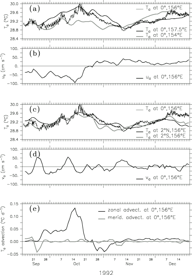
Figure 8. Horizontal heat advection at 0°, 156°E. Daily averaged time series of the (a) vertically averaged surface layer temperatures along the equator at 0°, 154°E; 0°, 156°E; and 0°, 157.5°E and (b) vertically averaged zonal velocity at 0°, 156°E. Daily averaged time series of the (c) vertically averaged temperatures along the 156°E longitude at 2°N, 156°E; 0°, 156°E; and 2°S, 156°E and (d) vertically averaged meridional velocity at 0°, 156°E. (e) Daily estimates of the zonal and meridional heat advection.
The convergence of heat due to stratified shear flow (terms in (2) involving
![]() )
cannot be measured with the array and is possibly nonnegligible. Likewise the
entrainment and turbulent diffusive mixing cannot be directly measured. Consequently,
the residual of the heat balance includes instrumental and sampling errors,
the convergence of heat due to stratified shear flow, entrainment mixing, and
turbulent diffusion. For the sake of argument, in the following section we will
most often interpret the residual as primarily due to entrainment mixing, with
the understanding that this is sometimes overly simplistic. However, independent
support for this basic interpretation will be provided in section 5, where the
residual is compared to entrainment mixing as parameterized by Niiler
and Kraus [1977].
)
cannot be measured with the array and is possibly nonnegligible. Likewise the
entrainment and turbulent diffusive mixing cannot be directly measured. Consequently,
the residual of the heat balance includes instrumental and sampling errors,
the convergence of heat due to stratified shear flow, entrainment mixing, and
turbulent diffusion. For the sake of argument, in the following section we will
most often interpret the residual as primarily due to entrainment mixing, with
the understanding that this is sometimes overly simplistic. However, independent
support for this basic interpretation will be provided in section 5, where the
residual is compared to entrainment mixing as parameterized by Niiler
and Kraus [1977].
All terms were filtered with a 5-day triangular filter (3-day cutoff) and subsampled
once per day. As shown in Table 4, the standard deviations of all terms in (2b)
are larger than the rms errors and therefore variability in the heat balance
can be resolved. Errors in the heat flux analysis (2b) are dominated by uncertainties
in the storage term (46 W m) due to uncertainties
in h and Ta. Errors in the net surface heat flux are
about 15 W m. When the heat balance is written
in terms of temperature tendency ((2a) instead of (2b)), errors are dominated
by the surface heat flux tendency rate ((Q
- Q)/ch)
primarily because of errors in h.
In describing our heat budget calculations in the following sections, we will
favor presentation in terms of the temperature tendency equation (2a) rather
than heat content equation (2b) since our target diagnostic variable is surface
layer temperature. However, for comparison, results are summarized for both
temperature tendencies and the temperature tendencies scaled by the layer heat
capacity ch.
Conclusions about the relative importance of various terms in the surface layer
balances are unaffected by the choice of diagnostic equation.
The heat fluxes are quite sensitive to variability in the wind speed (Tables 2-4) and therefore naturally group into a period before the westerly wind burst from the beginning of the deployment to October 17, a westerly wind burst period from October 18 to November 12, and a period following the wind burst from November 13 to December 7. Toward the end of the record, near December 8, another westerly wind burst began to develop (Figure 3a), but did not reach full strength until after the end of the deployment [Gutzler et al., 1994; Chen et al., 1996; Weller and Anderson, 1996].
From the beginning of the record until mid-October, the top of the thermocline
was quite shallow (Figure 4a), with the upper
layer depth (depth of the 21.8 surface)
generally between 20 and 40 m. Above the shallow pycnocline, the surface zonal
flow was westward (Figure 4d), associated with
the South Equatorial Current. The surface meridional flow was characterized
by ~15-day wavelike changes in speed and direction, with northward surface flow
occurring during two southerly wind episodes.
Between the two southerly wind episodes, there was nearly two weeks (September 25 to October 7) of relatively light wind and cloudless days during which the SST at 1 m depth had a strong diurnal cycle, varying by more than 1°C over the course of the day (Figure 7). During this quiescent period, the warm pool had a strong temperature gradient with higher SSTs east of 0°, 156°E (Figure 8a), and consequently the zonal heat advection at 0°, 156°E was nearly as large as the net surface heat flux (Figures 8e and 9).
During the period October 8-17, extended cloudiness and moderate winds caused the surface heat flux to be near zero (Figure 6). The upper layer, however, continued to warm by almost 0.8°C (Figure 7) due to extremely strong westward warm heat advection (Figures 8e and 9). Thus, as summarized in Figure 10a, during the period from September 19 to October 17, 1992, the upper ocean was warmed locally by shortwave radiation and by heat advection from the east and was to a lesser extent cooled by latent heat loss and vertical mixing.
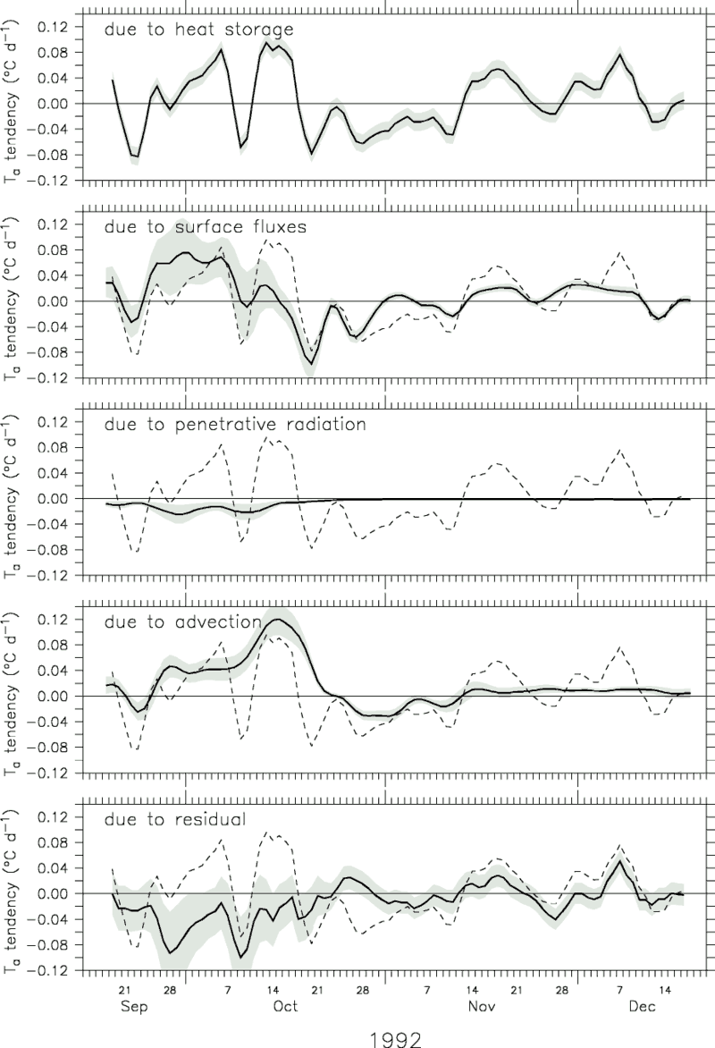
Figure 9. The 5-day triangular filtered surface layer heat balance
in units of degrees Celcius per day. The heat storage rate (Ta/t)
is repeated as a dashed line in each panel. The ±1 rms error for each term is
indicated by the shading.
In mid-October a series of three to four strong southwesterly wind episodes
occurred, each with wind speeds of roughly 7-8 m s.
Outgoing longwave radiation (OLR) observations [Gutzler
et al., 1994; Chen
et al., 1996] show that the increased cloudiness extended over
15°-20° of longitude and propagated eastward at approximately 1.5 m s.
These combined southwesterly episodes spanned approximately 26 days during which
the SST cooled by over 1°C. This period will be referred to hereafter as "the
October wind burst."
As a result of the decreased shortwave radiation and the enhanced latent heat loss, surface cooling occurred during daytime as well as nighttime. Persistent westerly winds accelerated the surface currents such that by the end of October, the surface equatorial jet completely reversed direction to become eastward. Consequently, the heat advection became a cooling process. As the warm advection decreased and the surface cooling increased, the SST began to steadily cool. During this cooling period, the SST diurnal cycle was suppressed; SST was nearly identical to (and for several particularly rainy hours even cooler than) the vertically averaged upper layer temperature (Figure 7).
As shown in Figure 4c, the ocean response to the westerly wind burst also included a deepening of the pycnocline of over 50 m. Analyses of the mass balance indicate that this deepening was due primarily to meridional Ekman convergence in the surface layer [R. Weisberg, personal communication, 1996] rather than to turbulent mixing. The slight warming in the residual term during October 21-25 cannot represent mixing since the thermocline was stably stratified. Thus during this westerly wind burst period from October 18 to November 12, 1992, the upper ocean cooled due to a net surface heat loss and to a lesser extent due to vertical mixing and eastward advection of cooler water (Figure 10b).
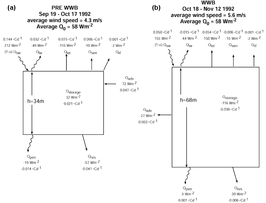
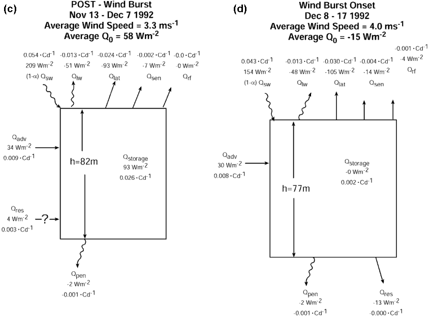
Figure 10. Box diagrams of the heat balance (equations (2a) and (2b)) for (a) the pre-wind burst period from September 19 to October 17, 1992, (b) the wind burst period from October 18 to November 12, 1992, (c) the post-wind burst period from November 13 to December 7, 1992, and (d) the beginning of the December wind burst from December 8 to 17, 1992. The mean wind speed during each period is listed, and the mean layer depth is indicated in the boxes. As discussed in the text, although we generally interpret the residual in terms of entrainment mixing, during the post-wind burst period the residual is positive and therefore cannot represent mixing. Instead, we believe that during this period it may represent horizontal advection of a sharp temperature front.
From mid-November through mid-December, winds were generally light (less than
4 m s), shortwave radiation was near the
clear-sky value, and precipitation was negligible. As shown in Figures
6 and 9, shortwave radiative warming dominated
over surface cooling fluxes. Likewise, as shown in Figure
8, the zonal temperature gradient and therefore heat advection changed sign,
becoming warm advection from the west. As a result of these warming processes,
the surface layer began to warm (Figures 9 and
10c).
During this post-wind burst period, the top of the pycnocline was quite deep (i.e., below 80 m). Near-surface restratification in the thermal field was evident in the latter part of November. However, higher salinity near the surface compensated for the thermal stratification, and consequently near-surface restratification is less evident in the density field. Thus the primary effect of this thermal restratification was to make the vertically averaged surface layer temperature, Ta, less of a SST proxy.
The intense December 5-7 warming in the residual (Figure
9) cannot be due to entrainment mixing because the temperature field associated
with the pycnocline was stably stratified. Since there was both near-surface
stratification and shear, it could possibly be due in part to the unresolved
terms in (2) involving ![]() .
Alternatively, the intense warming event could be due to the passage of a sharp
temperature front that was not adequately resolved by the mooring array. As
shown in Figure 8a, prior to December 5 the surface
layer temperatures at 0°, 156°E and 0°, 157.5°E were nearly identical and were
both approximately 0.4°C cooler than the surface layer water to the west at
0°, 154°E. Then, over the course of 3-4 days, the temperature of the surface
layer at 0°, 156°E increased by 0.4°C to become nearly identical to the temperature
at 0°, 154°E. With a 20 cm s zonal current,
a 0.4°C temperature change in 4 days corresponds to the passage of a front across
which temperature changes by 0.5°C in 70 km. Sharp fronts (0.4°C in 40 km) were
observed near 2°S, 156°E during COARE [Henin
et al., 1994]; however, further analysis of COARE data is needed
to determine if this large warming event at 0°, 156°E can be conclusively attributed
to zonal advection of a sharp temperature front.
.
Alternatively, the intense warming event could be due to the passage of a sharp
temperature front that was not adequately resolved by the mooring array. As
shown in Figure 8a, prior to December 5 the surface
layer temperatures at 0°, 156°E and 0°, 157.5°E were nearly identical and were
both approximately 0.4°C cooler than the surface layer water to the west at
0°, 154°E. Then, over the course of 3-4 days, the temperature of the surface
layer at 0°, 156°E increased by 0.4°C to become nearly identical to the temperature
at 0°, 154°E. With a 20 cm s zonal current,
a 0.4°C temperature change in 4 days corresponds to the passage of a front across
which temperature changes by 0.5°C in 70 km. Sharp fronts (0.4°C in 40 km) were
observed near 2°S, 156°E during COARE [Henin
et al., 1994]; however, further analysis of COARE data is needed
to determine if this large warming event at 0°, 156°E can be conclusively attributed
to zonal advection of a sharp temperature front.
As summarized in Figure 10c, warming during this post-wind burst period from November 13 to December 7, 1992, was caused by strong surface heat flux into the ocean and by warm eastward heat advection. Unlike during the pre-wind burst period when the pycnocline was shallow, mixing of cold (deep) pycnocline water into the upper ocean layer was negligible during the post-wind burst period.
On December 11, a short 3-day northwesterly wind burst occurred, and the surface layer temperature cooled due to the combined reduction in insolation, increase in latent heat loss, and increase in the residual processes (turbulent mixing). Prolonged precipitation events caused cool, freshwater anomalies in the surface (1 m) salinity, and associated subsurface temperature maxima at 10 m depth. The pycnocline, however, was located at approximately 60 m, well below the shallow subsurface temperature maximum (Figure 4a), so that the residual remained a weak cooling process. As the record ends, the winds began intensifying into the "December wind burst" which is the focus of much COARE research [e.g., Smyth et al., 1996; Weller and Anderson, 1996].
As shown in Figure 9, the residual of the heat budget is barely larger than its error (estimated through propagation of errors) and is therefore likely to involve more than just mixing. Thus we use a second, indirect method of estimating entrainment mixing using the turbulent energy balance. Assuming horizontally homogeneous and steady state turbulence in which the dissipation is proportional to the generation of turbulence, we have [Niiler and Kraus, 1977]
 |
(4) |
where w = dh/dt + w-h
is the entrainment velocity (w
= dh/dt + w-h
is the entrainment velocity (w
 0);
0);  b
= -g(
- -h)/0
is the buoyancy of the vertically averaged layer relative to the base of the
layer (g is gravity); h is the layer depth; Rib
= bh |v|
is the bulk Richardson number (v = v
b
= -g(
- -h)/0
is the buoyancy of the vertically averaged layer relative to the base of the
layer (g is gravity); h is the layer depth; Rib
= bh |v|
is the bulk Richardson number (v = v - v-h is the layer velocity relative to the base of
the layer); m, n, and s are empirically determined efficiency
factors; u* = (
- v-h is the layer velocity relative to the base of
the layer); m, n, and s are empirically determined efficiency
factors; u* = ( /)
/) is the frictional velocity ( is wind stress);
B is the surface buoyancy
flux due to heat and freshwater fluxes adjusted for the surface penetrative
radiation buoyancy flux J
(38% of the incoming shortwave radiation); and
is the frictional velocity ( is wind stress);
B is the surface buoyancy
flux due to heat and freshwater fluxes adjusted for the surface penetrative
radiation buoyancy flux J
(38% of the incoming shortwave radiation); and  is the extinction depth (taken to be 22.1 m). Following Niiler and Kraus, we
assume a single exponential for the penetrative radiation in deriving (4) since
for h >>> 1 m, the first term in (3) is essentially zero. Note,
however, that our (4) differs from Niiler
and Kraus [1977] by the inclusion of the term (h + 2)
J e-h,
which can be large when h
is the extinction depth (taken to be 22.1 m). Following Niiler and Kraus, we
assume a single exponential for the penetrative radiation in deriving (4) since
for h >>> 1 m, the first term in (3) is essentially zero. Note,
however, that our (4) differs from Niiler
and Kraus [1977] by the inclusion of the term (h + 2)
J e-h,
which can be large when h  -1
~ 22 m.
-1
~ 22 m.
The efficiency factors m, n, and s express how much of the turbulence is dissipated within the layer rather than entrained across the layer depth. A value of m = 0, n = 0, or s = 0 would mean that all turbulence generated by wind stirring, free convection, or shear instability, respectively, is dissipated and unavailable for entrainment mixing. Consequently, the layer depth would be a material surface. As discussed by McPhaden [1982], the s parameter can be interpreted as a critical bulk Richardson number, above which shear production is effectively dissipated.
The Niiler-Kraus entrainment velocity is calculated from (4) using hourly data. As with the surface layer heat balance, the hourly estimate of entrainment cooling is then filtered with a 5-day triangular filter and subsampled once per day. Figure 11a shows the tendency rates for the three cases of purely wind-generated turbulence (m = 1, n = 0, s = 0), purely buoyancy-driven turbulence (m = 0, n = 1, s = 0), and purely shear-generated turbulence (m = 0, n = 0, s = 1). As one might expect from the strong correlation between surface fluxes and wind speed, the mixing rates due to wind stirring are quite similar to the mixing rate due to free convection, although free convection is a more efficient source of turbulence than the wind stirring. Shear-generated turbulence, on the other hand, is an extremely efficient source of turbulence only when the shear is sufficiently strong and the relative buoyancy is sufficiently low. At other times, the shear-generated turbulence is negligible.
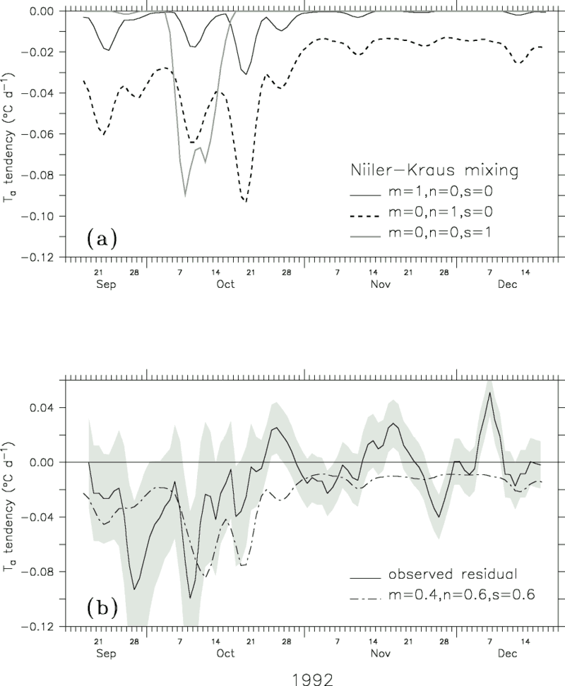
Figure 11. (a) Niiler and Kraus's [1977] parameterization of the entrainment mixing rate for the three cases of pure wind-generated turbulence (m = 1, n = 0, s = 0), pure free convection (m = 0, n = 1, s = 0), and pure shear-generated turbulence (m = 0, n = 0, s = 1). (b) Time series of the heat balance residual (solid curve) and the optimized Niiler-Kraus entrainment mixing rate (m = 0.4, n = 0.6, s = 0.6) (dashed curve). The heat balance residual includes entrainment mixing, diffusion, heat convergence due to the stratified and shear flow, and errors. The rms error of the observed residual is indicated by shading.
To determine the optimal empirical values, mixing rates were evaluated for the parameter range m = 0 - 2, n = 0 - 1, and s = 0 - 1. The 5-day filtered and subsampled mixing rates were then compared to the observed residual tendency rate for periods in which the 5-day filtered residual tendency rate was negative (primarily during the first month of the record). During this period, the mixing rate with parameters m = 0.4, n = 0.6, and s = 0.6 was found to have the minimal mean and rms difference and maximum correlation with the observed residual tendency rate. This optimal Niiler-Kraus mixing rate and the observed residual tendency rate are shown in Figure 11b. Both the large errors and the simplicity of the Niiler-Kraus parameterization preclude a detailed comparison. Nevertheless, as can be seen in Figure 11b, both time series imply higher mixing rates in September and October when the pycnocline was shallow, and lower mixing rates in November and December when the pycnocline was deep. Relatively low values of parameterized turbulent entrainment in late October indicate that the deepening of the pycnocline at that time (Figure 4c) was not due to turbulent mixing. This is consistent with our interpretation that the deepening is due to westerly wind-driven meridional Ekman convergence in the surface layer.
SST in the warm pool is relatively homogenous in comparison to other regions of the equatorial Pacific, and therefore traditionally it has been assumed that one-dimensional models should be able to simulate temperature fairly well in this region. Our analysis of the thermal response at 0°, 156°E, however, shows that heat advection can be at times a dominant heating mechanism, as, for example, prior to and during the early stage of the October 1992 wind burst and possibly in early December. Furthermore, since the heat storage and entrainment cooling rates depend upon the layer depth, the upper layer heat balance is affected by three-dimensional processes such as Ekman convergence and divergence that result in variability in the pycnocline depth. To further investigate the effects of these three-dimensional processes, the observations will be compared to a one-dimensional model simulation.
The Price-Weller-Pinkel ("PWP") [Price
et al., 1986] mixed layer model will be used for the one-dimensional
simulation. The PWP model is initialized with CTD and ADCP data at the mooring
site from September 15, 1995. The temperature, salinity, and momentum within
the top vertical level (z = 20 cm) are then integrated forward one time
step (1 hour) by absorbing the observed shortwave radiation using the Siegel
double exponential profile (3) and by applying the observed longwave radiation
and turbulent heat flux, evaporation minus precipitation, and wind stress as
surface boundary conditions for the one-dimensional heat, salinity, and momentum
equations. Additionally, a linear drag function (-Cu) with an e-folding
timescale of 7 days is included in the momentum balance to account for unresolved
dynamics. As will be discussed later, without this linear drag the surface equatorial
currents become unrealistically large. The temperature and salinity profiles
are then combined to form a density profile, assuming constant thermal expansion
and haline contraction coefficients. Temperature, salinity, and velocity profiles
are mixed down each vertical step of 20 cm until the three stability criteria
are satisfied: (1) convective stability (-/z
0); (2) mixed layer stability (bulk Richardson
number = -gh-1
|v |
0.65); and (3) shear flow stability (gradient
Richardson number = -g
/z
|v/z|
0.25).
As shown in Figure 12a, by the end of the 3-month record the one-dimensional simulated SST is nearly 0.8°C cooler than the observed SST. Much of this drift occurs during the second week of October (Figures 12a and 12b), precisely when zonal advection dominated the observed heat balance (Figure 9). The deepening of the thermocline during the October wind burst is not captured (Figure 13), consistent with our interpretation that the deepening is due to dynamical processes rather than turbulent erosion of the pycnocline. Thus the differences between the observed and one-dimensional simulated low-frequency tendency rates can be interpreted as due to "missing" three-dimensional processes in the upper ocean heat, mass, and momentum balances. On the other hand, the simulated SST variability on timescales less than 5 days is correlated quite well (0.9) with the observed 5-day high-passed SST (Figure 12c). The diurnal cycle is determined primarily by daytime warming due to shortwave radiation, and nighttime turbulent mixing similar to that found in the eastern equatorial Pacific [Bond and McPhaden, 1995]. Thus diurnal variations are more reasonably described by a one-dimensional balance in the warm pool.
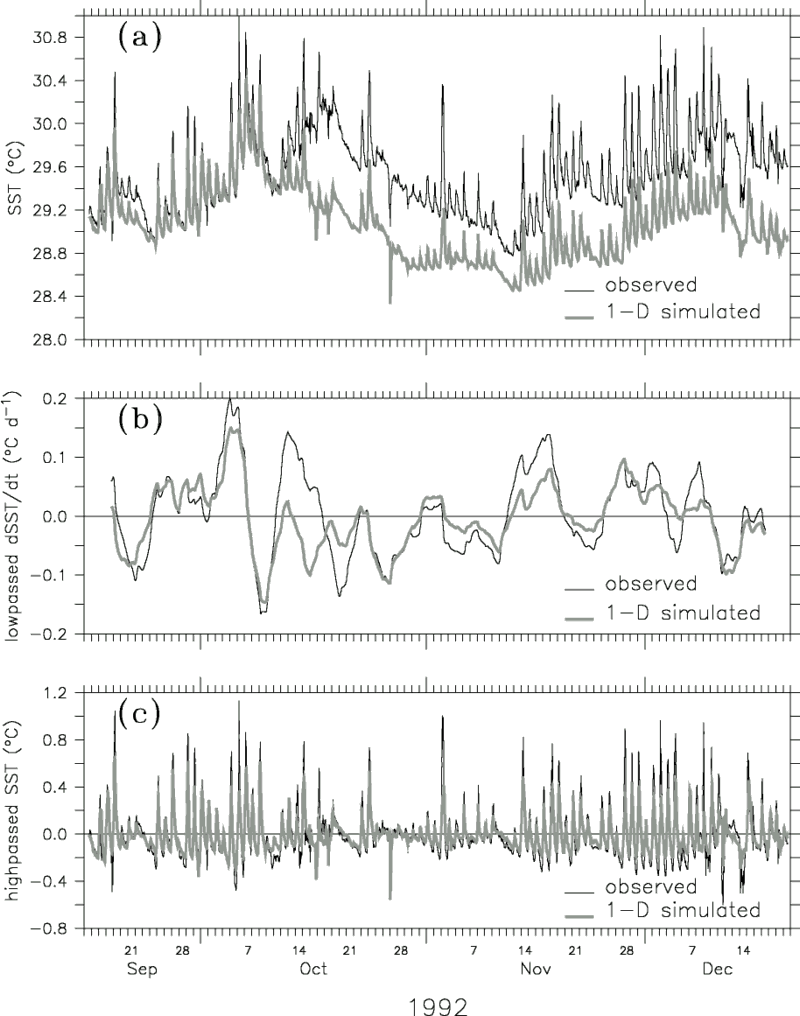
Figure 12. Price-Weller-Pinkel one-dimensional mixed layer simulation at 0°, 156°E from September 17 to December 20, 1992. (a) Observed SST (thin curve) and simulated SST (thick curve) at 1 m depth. (b) The 5-day triangular filtered observed SST tendency rate (thin curve) and simulated SST tendency rate (thick curve). (c) The 5-day high-passed SST (thin curve) and simulated SST (thick curve).
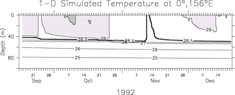
Figure 13. Daily averaged PWP simulated temperature stratification. The CIs are the same as in Figure 4a.
We note that when the model was run without the linear drag in the momentum
equation, the winds generated surface currents with speeds of up to 180 cm s.
Consequently, the surface temperatures cooled by an additional 1°C over the
3-month period due to the increased vertical entrainment. This "no drag"
run is not realistic because of the intense current velocities generated. However,
it gives an indication of the sensitivity of the one-dimensional model simulations
to parameter variations.
On diurnal timescales and to a large extent even on longer timescales, the warm pool's SST variability is controlled by variability in the insolation and latent heat loss. During wind bursts, reduced insolation and increased latent heat loss tend to cool the upper ocean temperature, while during quiescent periods (periods of suppressed atmospheric convection), increased insolation and reduced latent heat loss tend to warm the upper ocean temperature. An important result of this analysis, however, is that horizontal heat advection can also be a dominant process controlling SST variability.
Horizontal heat advection requires a horizontal current oriented along a temperature
gradient. While the long-term mean surface currents and temperature gradients
in this region are small, wind forcing due to the easterly trades, modulated
by westerly wind bursts, can cause large O(50 cm s)
equatorially trapped surface currents which can be either westward or eastward
depending upon the forcing. The time-longitude plot of the equatorial Pacific
SST [Reynolds
et al., 1994] for January 1991 through December 1994 (Figure
14) indicates that at 0°, 156°E the zonal temperature gradient is generally
positive (warmer water to the east, cooler water to the west). A simple scale
analysis can determine how large the temperature gradient must be to produce
substantial heat advection: throughout the entire 4-year period, the weekly
SST at 0°, 156°E never varied by more than 1.5°C, although during warming and
cooling events SST varied by up to ±1°C month.
For a 50 cm s zonal current to produce a
1°C SST change in 1 month by zonal advection, an SST gradient of 1°C in 1300
km or approximately 12° of longitude would be required. Temperature gradients
of this magnitude are not uncommon in the warm pool, as can be seen in Figure
14 (e.g., September-October 1991, September-October 1992, and August-October
1993). Additionally, although not resolved by the weekly 1° × 1° SST fields,
sharp temperature fronts, such as those observed during COARE, could also result
in significant SST variability due to advection. Thus the warm pool surface
currents and temperature gradients are potentially large enough to make horizontal
heat advection an order one process in the time-varying heat balance.

Figure 14. Time-longitude plot of the Reynolds et al. [1994] SST from January 1991 through December 1994, along the equator (average of 0.5°S and 0.5°N) from 140°E to 110°W. The study period is highlighted by a line along the left edge of the time axis. Likewise the study region is highlighted by line through the contoured time series at 0°, 156°E. The CI is 1°C and 0.5°C for SST values less than and greater than 28°C, respectively. The 28.5°C contour (dark line) indicates the boundary of the warm pool.
Using 4 years of data from 250 surface drifters in the western equatorial Pacific, Ralph et al. [1997] show that while advection by the long-term mean current is negligible, long-term mean advection is not. On average, eastward surface currents tend to be correlated with an increased positive temperature gradient, and thus the variable currents and temperature gradients result in a net long-term heat advection which is a cooling process in the warm pool. The correlation in this case is due to westerly wind bursts which tend both to produce eastward surface jets and to increase the temperature gradient by cooling the SST in the western portion of the warm pool (where wind speeds and, presumably, evaporative cooling associated with wind bursts are larger). It should be noted, however, that the statistical range of variability in their analysis also includes westward warm advection events such as we observed in October 1992. During this event, the westward South Equatorial Current and a positive temperature gradient combined to produce substantial warming at 0°, 156°E. Instantaneously as well as climatologically, heat advection events are important in the warm pool's heat balance.
The dependence of entrainment cooling on the depth of the thermocline causes a further complication to the simple one-dimensional heat balance. On the basis of the turbulent energy budget and the empirical three-dimensional heat balance (Figure 11), the strength of entrainment cooling depends upon the location of the reservoir of cold water relative to the source of turbulence. When the thermocline is shallow, as it was in September and early October 1992, turbulent entrainment mixing can be an important cooling process in the upper ocean heat balance. The 2.5-year time series of temperature as a function of depth at 0°, 156°E (Figure 15) shows that from February through October 1992 and again from July through October 1993 the thermocline was extremely shallow. One might expect that during these times entrainment cooling was potentially large. In contrast, throughout the COARE IOP (November 1992 to February 1993), the thermocline was below 70 m and one might expect that entrainment cooling was reduced during this period. Indeed, Anderson et al. [1996] show that for much of the COARE IOP the upper ocean temperature tendency was in near-balance with the surface heat flux rate (see their Figure A1).
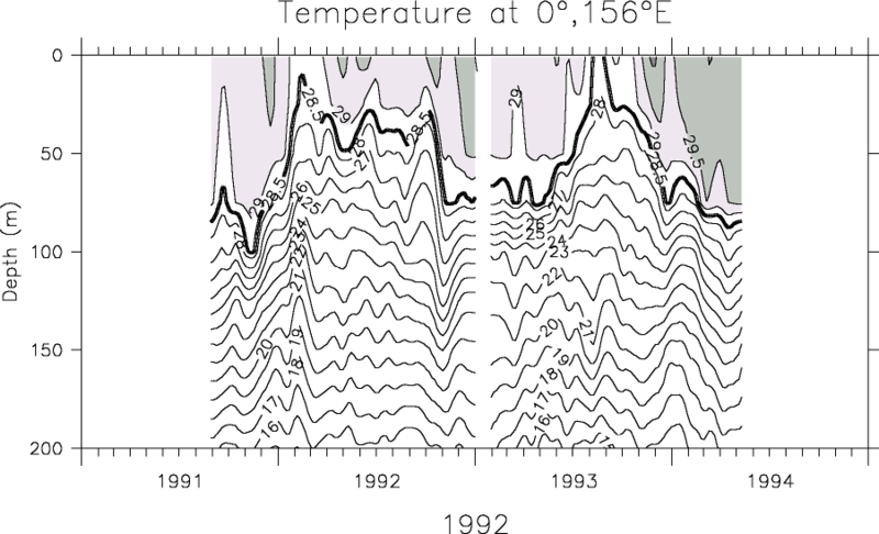
Figure 15. Time series of the subsurface temperature profile at 0°, 156°E. Data have been low passed with a 29-day triangular filter. The CIs are the same as in Figure 4a.
While the deepening of the pycnocline in October 1992 occurred as a dynamical response to the October 1992 westerly wind burst, as can be seen in Figure 15, not all westerly wind bursts have this response. The differences are due to the fact that pycnocline responses to wind burst forcing in general depend not only on local Ekman convergence but also on the excitation of equatorial waves, most notably Kelvin and Rossby waves. Previous studies have shown that the mix of local wind forcing and remote forcing at a particular location in the warm pool can lead to a variety of responses (upwelling, downwelling, or more complicated evolutions) [e.g., McPhaden et al., 1990, 1992; Delcroix et al., 1993]. The details of the response depend on the space/time structure of the wind forcing, the location of the observational array relative to the forcing region, and oceanic initial conditions on which that forcing operates.
Upper ocean stratification can also be affected by high levels of precipitation in the warm pool region. In particular Lukas and Lindstrom [1991] hypothesized that heavy precipitation in the western Pacific can lead to the formation of a barrier layer, i.e., a salt-stratified layer between the bottom of the surface isopycnal layer and the top of the thermocline. Using CTD data from the western equatorial Pacific, Ando and McPhaden [1997] found that during COARE the barrier layer was on average about 10 m thick. With the vertical resolution of the moored time series data (Table 1), this thickness is at the margins of detection. Nevertheless, during a period of persistent rain in the second week of December, short-lived, shallow barrier layers greater than 10 m thick were observed in the 0°, 156°E moored data. As can be seen in Figures 4a and 7, during these events the stability of the surface freshwater stratification was at times enough to support temperature inversions such that the SST was cooler than subsurface temperatures. Similar short-lived, shallow barrier layers were observed at 2°S, 156°E during the COARE IOP [Anderson et al., 1996; Smyth et al., 1996; Huyer et al., 1997]. Using a one-dimensional mixed layer model, Anderson et al. [1996] show that the SST cooling and subsequent temperature inversions associated with these shallow barrier layers are due in part to the increased loss of penetrating shortwave radiation across the base of the mixed layer. For barrier layers deeper than the shortwave extinction depth (~25 m), reduced entrainment mixing should result in warmer SSTs, consistent with the Lukas and Lindstrom [1991] hypothesis. A more complete understanding of the climatic impacts of barrier layer variations will require analyses of ocean-atmosphere interactions involving the long-term, large-scale hydrological cycle in and over the ocean, work which is currently underway.
This study represents one of the first analyses in which the full three-dimensional heat balance of the western equatorial Pacific warm pool has been estimated on timescales associated with westerly wind burst forcing in the western equatorial Pacific warm pool. The analysis is based on unique in situ time series measurements collected during TOGA-COARE to determine surface heat fluxes, upper ocean temperature and salinity variability, and upper ocean currents. These data have allowed for a quantitative assessment of the processes affecting SST, a variable of significant climatic importance in the coupled ocean-atmosphere system.
The variability in the heat balance observed during the 3-month study period highlights the fact that long time series are required to obtain mean values of sources and sinks of heat in the warm pool. As discussed in section 4 and shown in Figures 6, 9, and 10, over the course of a wind burst the net surface heat flux can change sign, being a warming process prior to and following the wind burst, and an equally strong cooling process during the wind burst. Horizontal heat advection also is highly variable due to variations in the temperature gradients and reversals in the surface current direction. Additionally, the depth of the thermocline has variability that affects entrainment cooling and heat storage rate. Thus, high-quality data obtained during COARE within the framework of the TAO enhanced monitoring array have provided an ideal data set for analyzing the complexity of these and related processes involved in the surface layer heat balance in the western equatorial Pacific warm pool.
Acknowledgments. This research was supported by NOAA's Office of Global Programs and by a UCAR Visiting Scientist Programs' NOAA Climate and Global Change postdoctoral award to M. Cronin. We would like to thank H. P. Freitag for his assistance in processing the data, and the TAO operational group for their dedicated work in obtaining high-quality routine measurements. Special thanks go to the chief scientist, Thierry Delcroix of ORSTOM, Noumea, and the crew of the R/V Le Noroit, who rescued the errant 0°, 156°E PROTEUS buoy on Christmas Eve, 1992. Additionally we would like to thank D. E. Harrison, several members of the COARE air-sea flux group (D. Rogers, O. Tsukamoto, S. Anderson, F. Bradley, C. Fairall, B. Weller), and the COARE heat budget subgroup (B. Smyth, D. Siegel, C. Ohlmann, H. Wijesekera, E. Antonissen, S. Godfrey) for particularly helpful discussions of this work. This is PMEL contribution 1713.
Anderson, S. P., R. A. Weller, and R. B. Lukas, Surface buoyancy forcing and the mixed layer of the western Pacific warm pool: Observations and 1-d model results, J. Clim., 9, 3056-3085, 1996.
Ando, K., and M. J. McPhaden, Variability of surface layer hydrography in the tropical Pacific ocean, J. Geophys. Res., in press, 1997.
Barnett, T. P., An attempt to verify some theories of El Nińo, J. Phys. Oceanogr., 7, 633-647, 1977.
Bjerknes, J., Atmospheric teleconnections from the equatorial Pacific, Mon. Weather Rev., 97, 163-172, 1969.
Bond, N. A., and M. J. McPhaden, An indirect estimate of the diurnal cycle in the upper ocean turbulent heat fluxes at the equator, J. Geophys. Res., 100, 18,369-18,378, 1995.
Chen, S. S., R. A. Houze Jr., and B. E. Mapes, Multiscale variability of deep convection in relation to large-scale circulation in TOGA COARE, J. Atmos. Sci., 53, 1380-1409, 1996.
Clark, N. E., L. Eber, R. M. Laurs, J. A. Renner, and J. F. T. Saur, Heat exchange between ocean and atmosphere in the eastern North Pacific for 1961-71, NOAA Tech. Rep. NMFS SSRF-682, U.S. Dep. Commer., Washington, D.C., 1974.
Delcroix, T., G. Eldin, M. McPhaden, and A. Morliére, Effects of westerly wind bursts upon the western equatorial Pacific Ocean, February-April 1991, J. Geophys. Res., 98, 16,379-16,385, 1993.
Fairall, C., E. F. Bradley, D. P. Rogers, J. B. Edson, and G. S. Young, Bulk parameterization of air-sea fluxes for Tropical Ocean-Global Atmosphere Coupled-Ocean Atmosphere Response Experiment algorithm, J. Geophys. Res., 101, 3747-3764, 1996a.
Fairall, C., E. F. Bradley, J. S. Godfrey, G. A. Wick, J. B. Edson, and G. S. Young, Cool skin and warm layer effects on sea surface temperature, J. Geophys. Res., 101, 1295-1308, 1996b.
Fofonoff, P., and R. C. Millard Jr., Algorithms for computation of fundamental properties of seawater, Tech. Pap. Mar. Sci., 44, 53 pp., Unesco, Paris, 1983.
Freitag, H. P., Y. Feng, L. J. Mangum, M. J. McPhaden, J. Neander, and L. D. Stratton, Calibration procedures and instrumental accuracy estimates of TAO temperature, relative humidity and radiation measurements. NOAA Tech. Memo. ERL PMEL-104, 32 pp., Pac. Mar. Environ. Lab., NOAA, Seattle, Wash., 1994.
Fung, I. Y., D. E. Harrison, and A. A. Lacis, On the variability of the net longwave radiation at the ocean surface, Rev. Geophys., 22, 177-193, 1984.
Godfrey, J. S., and E. J. Lindstrom, The heat budget of the equatorial western Pacific surface mixed layer, J. Geophys. Res., 94, 8007-8017, 1989.
Graham, N. E., and T. P. Barnett, Sea surface temperature, surface wind divergence, and convection over tropical oceans, Science, 238, 657-659, 1987.
Gutzler, D. S., G. N. Kiladis, G. A. Meehl, K. M. Weickmann, and M. Wheeler, The global climate of December 1992-February 1993, II, Large-scale variability across the tropical western Pacific during TOGA COARE, J. Clim., 7, 1606-1622, 1994.
Harrison, D. E., and B. S. Giese, Episodes of surface westerly winds as observed from islands in the western tropical Pacific, J. Geophys. Res., 96, suppl., 3221-3237, 1991.
Henin, C., J. Grelet, and M.-J. Langlade, Observations intensives de la température et de la salinité de surface dans le Pacifique tropical ouest entre 20°S et 20°N (1991-1993), Arch. Sci. Mer Océanogr. Phys. 8, 75 pp., Inst. Fr. de Rech. Sci. pour le Dev. en Coop. (ORSTOM), Nouméa, New Caledonia, 1994.
Huyer, A., P. M. Kosro, R. Lukas, and P. Hacker, Upper-ocean thermohaline fields near 2°S, 156°E during TOGA-COARE, November 1992 to February 1993, J. Geophys. Res., in press, 1997.
Kessler, W. S., M. J. McPhaden, and K. M. Weickmann, Forcing of intraseasonal Kelvin waves in the equatorial Pacific, J. Geophys. Res., 100, 10,613-10,631, 1995.
Lien, R.-C., M. J. McPhaden, and D. Hebert, Intercomparison of ADCP measurements at 0°, 140°W. J. Atmos. Oceanic Technol., 11, 1334-1349, 1994.
Liu, W. T., K. B. Katsaros, and J. A. Businger, Bulk parameterization of air-sea exchanges of heat and water vapor including the molecular constraints at the interface, J. Atmos. Sci., 36, 1722-1735, 1979.
Lukas, R., and E. Lindstrom, The mixed layer of the western equatorial Pacific Ocean, J. Geophys. Res., 96, suppl., 3343-3357, 1991.
Luther, D. S., D. E. Harrison, and R. A. Knox, Zonal winds in the central equatorial Pacific and El Nińo, Science, 222, 327-330, 1983.
McCarty, M. E., and M. J. McPhaden, Mean seasonal cycles and interannual variations at 0°, 165°E during 1986-1992, NOAA Tech. Memo. ERL PMEL-98, 64 pp., Pac. Mar. Environ. Lab., NOAA, Seattle, Wash., 1993.
McPhaden, M. J., Variability in the central equatorial Indian Ocean, II, Oceanic heat and turbulent energy balances, J. Mar. Res., 40, 403-419, 1982.
McPhaden, M. J., TOGA-COARE Optical Rain Gauge Measurements. Workshop Report, Seattle, Washington, 31 March-1 April 1993, TOGA Notes, no. 13, pp. 18-19, Nova Southeastern Univ. Oceanogr. Cent., Dania, Fla., 1993a.
McPhaden, M. J., TOGA-TAO and the 1991-93 El Nińo-Southern Oscillation event, Oceanography, 6, 36-44, 1993b.
McPhaden, M. J., and S. P. Hayes, On the variability of winds, sea surface temperature, and surface layer heat content in the western equatorial Pacific. J. Geophys. Res., 96, 3331-3342, 1991.
McPhaden, M. J., and H. B. Milburn, Moored precipitation measurements for TOGA, TOGA Notes, no. 7, pp. 1-5, Nova Southeastern Univ. Oceanogr. Cent., Dania, Fla., 1992.
McPhaden, M. J., H. P. Freitag, S. P. Hayes, B. A. Taft, Z. Chen, and K. Wyrtki, The response of the equatorial Pacific Ocean to a westerly wind burst in May 1986, J. Geophys. Res., 93, 10,589-10,603, 1988.
McPhaden, M. J., S. P. Hayes, L. J. Mangum, and J. M. Toole, Variability in the western equatorial Pacific during the 1986-87 El Nińo-Southern Oscillation event, J. Phys. Oceanogr., 20, 190-208, 1990.
McPhaden, M. J., F. Bahr, Y. Du Penhoat, E. Firing, S. P. Hayes, P. P. Niiler, P. L. Richardson, and J. M. Toole, The response of the western equatorial Pacific Ocean to westerly wind bursts during November 1989 to January 1990, J. Geophys. Res., 97, 14,289-14,303, 1992.
Meyers, G., J.-R. Donguy, and R. K. Reed, Evaporative cooling of the western equatorial Pacific Ocean by anomalous winds, Nature, 323, 523-526, 1986.
Miller, L., R. Cheney, and B. Douglas, Geosat altimeter observations of Kelvin waves and the 1986-87 El Nińo, Science, 239, 52-54, 1988.
Niiler, P. P., and E. B. Kraus, One-dimensional models of the upper ocean, in Modelling and Prediction of the Upper Layers of the Ocean, edited by E. B. Kraus, pp. 143-172, Pergamon, Tarrytown, N.Y., 1977.
Palmer, T. N., and D. A. Mansfield, Response of two atmospheric general circulation models to sea surface temperature anomalies in the tropical east and west Pacific, Nature, 310, 483-485, 1984.
Price, J., R. Weller, and R. Pinkel, Diurnal cycling: Observations and models of upper ocean response to diurnal heating, cooling and wind mixing, J. Geophys. Res., 91, 8411-8427, 1986.
Ralph, E. A., K. Bi, P. P. Niiler, and Y. du Penhoat, A Lagrangian description of the western equatorial Pacific response to the wind burst of December 1992: Heat advection in the warm pool, J. Clim., in press, 1997.
Reed, R., On estimating insolation over the ocean, J. Phys. Oceanogr., 7, 482-485, 1977.
Reynolds, R. W., D. C. Stokes, and T. M. Smith, A high-resolution global sea surface temperature analysis and climatology, TOGA Notes, no. 17, pp. 1-3, Nova Southeastern Univ. Oceanogr. Cent., Dania, Fla., 1994.
Siegel, D. A., J. C. Ohlmann, L. Washburn, R. R. Bidigare, C. T. Nosse, E. Fields, and Y. Zhou, Solar radiation, phytoplankton pigments and the radiant heating of the equatorial Pacific warm pool, J. Geophys. Res., 100, 4885-4891, 1995.
Smyth, W. D., D. Hebert, and J. N. Moum, Local ocean response to a multiphase westerly windburst, 2, Thermal and freshwater responses, J. Geophys. Res., 101, 22,513-22,533, 1996.
Sprintall, J., and M. McPhaden, Surface layer variations observed in multiyear time series measurements from the western equatorial Pacific, J. Geophys. Res., 99, 963-979, 1994.
Stevenson, J. W. and P. P. Niiler, Upper ocean heat budget during the Hawaii-to-Tahiti shuttle experiment, J. Phys. Oceanogr., 13, 1894-1907, 1983.
Thiele, O. W., M. J. McPhaden, and D. A. Short, Optical rain gauge performance, Proceedings of the Second Workshop on Optical Rain Gauge Measurements, NASA Conf. Publ., 3288, 76 pp., 1994.
Wang, T., and J. D. Crosby, Taking rain gauges to sea, Sea Tech., 34(12), 62-65, 1993.
Webster, P. J., and R. Lukas, TOGA COARE: The Coupled Ocean-Atmosphere Response Experiment, Bull. Am. Meteorol. Soc., 73, 1377-1417, 1992.
Weller, R. A., and S. P. Anderson, Temporal variability and mean values of the surface meteorology and air-sea fluxes in the western equatorial Pacific warm pool during TOGA COARE, J. Clim., 9, 1959-1990, 1996.
Zhang, C., Atmospheric intraseasonal variability at the surface in the tropical western Pacific Ocean, J. Atmos. Sci., 53, 739-758, 1996.
Zhang, G. J., and M. J. McPhaden, The relationship between sea surface temperature and latent heat flux in the equatorial Pacific, J. Clim., 8, 589-605, 1995.
Return to Abstract