Uptake and Storage of Carbon Dioxide in the Ocean: The Global CO₂ Survey

Richard A. Feely¹, Christopher L. Sabine², Taro Takahashi³, and Rik Wanninkhof⁴

¹Pacific Marine Environmental Laboratory, National Oceanic and Atmospheric Administration, Seattle, Washington, 98115
²Joint Institute for the Study of the Atmosphere and Ocean, University of Washington, Seattle, Washington, 98195
³Lamont-Doherty Earth Observatory, Palisades, New York
⁴Atlantic Oceanographic and Meteorological Laboratory National Oceanic and Atmospheric Administration, Miami, Florida

Oceanography, 14(4), 18–32 (2001).
Copyright ©2001 by The Oceanography Society. Further electronic distribution is not allowed.

Introduction

Human activity is rapidly changing the composition of the earth's atmosphere, contributing to warming from excess carbon dioxide (CO) along with other trace gases such as water vapor, chlorofluorocarbons, methane and nitrous oxide. These anthropogenic "greenhouse gases" play a critical role in controlling the earth's climate because they increase the infrared opacity of the atmosphere, causing the surface of the planet to warm. The release of CO from fossil fuel consumption or the burning of forests for farming or pasture contributes approximately 7 petagrams of carbon (1 Pg C = 1 × 10 g C) to the atmosphere each year. Approximately 3 Pg C of this "anthropogenic CO" accumulates in the atmosphere annually, and the remaining 4 Pg C is stored in the terrestrial biosphere and the ocean.

Where and how land and ocean regions vary in their uptake of CO from year to year is the subject of much scientific research and debate. Future decisions on regulating emissions of greenhouse gases should be based on more accurate models of the global cycling of carbon and the regional sources and sinks for anthropogenic CO, models that have been adequately tested against a well-designed system of measurements. The construction of a believable present-day carbon budget is essential for the reliable prediction of changes in atmospheric CO and global temperatures from available emissions scenarios.

The ocean plays a critical role in the global carbon cycle as a vast reservoir that exchanges carbon rapidly with the atmosphere, and takes up a substantial portion of anthropogenically-released carbon from the atmosphere. A significant impetus for carbon cycle research over the past several decades has been to achieve a better understanding of the ocean's role as a sink for anthropogenic CO. There are only three global reservoirs with exchange rates fast enough to vary significantly on the scale of decades to centuries: the atmosphere, the terrestrial biosphere and the ocean. Approximately 93% of the carbon is located in the ocean, which is able to hold much more carbon than the other reservoirs because most of the CO that diffuses into the oceans reacts with seawater to form carbonic acid and its dissociation products, bicarbonate and carbonate ions (Figure 1).

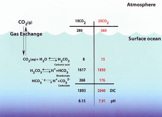
Figure 1. Schematic diagram of the carbon dioxide (CO) system in seawater. The 1 × CO concentrations are for a surface ocean in equilibrium with a pre-industrial atmospheric CO level of 280 ppm. The 2 × CO concentrations are for a surface ocean in equilibrium with an atmospheric CO level of 560 ppm. Current model projections indicate that this level could be reached sometime in the second half of this century. The atmospheric values are in units of ppm. The oceanic concentrations, which are for the surface mixed layer, are in units of µmol kg.

Our present understanding of the temporal and spatial distribution of net CO flux into or out of the ocean is derived from a combination of field data, which is limited by sparse temporal and spatial coverage, and model results, which are validated by comparisons with the observed distributions of tracers, including natural carbon-14 (C), and anthropogenic chlorofluorocarbons, tritium (H) and bomb C. The latter two radioactive tracers were introduced into the atmosphere-ocean system by atomic testing in the mid 20th century. With additional data from the recent global survey of CO in the ocean (1991–1998), carried out cooperatively as part of the Joint Global Ocean Flux Study (JGOFS) and the World Ocean Circulation Experiment (WOCE) Hydrographic Program, it is now possible to characterize in a quantitative way the regional uptake and release of CO and its transport in the ocean. In this paper, we summarize our present understanding of the exchange of CO across the air-sea interface and the storage of natural and anthropogenic CO in the ocean's interior.

Background

The history of large-scale CO observations in the ocean date back to the 1970s and 1980s. Measurements of the partial pressure of CO (pCO), total dissolved inorganic carbon (DIC) and total alkalinity (A) were made during the global Geochemical Ocean Sections (GEOSECS) expeditions between 1972 and 1978, the Transient Tracers in the Oceans (TTO) North Atlantic and Tropical Atlantic Surveys in 1981–83, the South Atlantic Ventilation Experiment (SAVE) from 1988–1989, the French Southwest Indian Ocean experiment, and numerous other smaller expeditions in the Pacific and Indian Oceans in the 1980s. These studies provided marine chemists with their first view of the carbon system in the global ocean.

These data were collected at a time when no common reference materials or standards were available. As a result, analytical differences between measurement groups were as large as 29 µmol kg for both DIC and A, which corresponds to more than 1% of the ambient values. Large adjustments had to be made for each of the data sets based on deepwater comparisons at nearby stations before individual cruise data could be compared. These differences were often nearly as large as the anthropogenic CO signal that investigators were trying to determine (Gruber et al., 1996). Nevertheless, these early data sets made up a component of the surface ocean pCO measurements for a global climatology and also provided researchers with new insights into the distribution of anthropogenic CO in the ocean, particularly in the Atlantic Ocean.

At the onset of the Global Survey of CO in the Ocean (Figure 2), several events took place in the United States and in international CO measurement communities that significantly improved the overall precision and accuracy of the large-scale measurements. In the United States, the CO measurement program was co-funded by the Department of Energy (DOE), the National Oceanic and Atmospheric Administration (NOAA) and the National Science Foundation (NSF) under the technical guidance of the U.S. CO Survey Science Team. This group of academic and government scientists adopted and perfected the recently developed coulometric titration method for DIC determination that had demonstrated the capability to meet the required goals for precision and accuracy. They advocated the development and distribution of certified reference materials (CRMs) for DIC, and later for A, for international distribution under the direction of Andrew Dickson of Scripps Institution of Oceanography (see sidebar). They also supported a shore-based intercomparison experiment under the direction of Charles Keeling, also of Scripps. Through international efforts, the development of protocols for CO analyses were adopted for the CO survey. The international partnerships fostered by JGOFS resulted in several intercomparison CO exercises hosted by France, Japan, Germany and the United States. Through these and other international collaborative programs, the measurement quality of the CO survey data was well within the measurement goals of ±3 µmol kg and ±5 µmol kg, respectively, for DIC and A.

Figure 2. The Global Survey of CO in the Ocean: cruise tracks and stations occupied between 1991 and 1998.

Several other developments significantly enhanced the quality of the CO data sets during this period. New methods were developed for automated underway and discrete pCO measurements. An extremely precise method for pH measurements based on spectrophotometry was also developed by Robert Byrne and his colleagues at the University of South Florida. These improvements ensured that the internal consistency of the carbonate system in seawater could be tested in the field whenever more than two components of the carbonate system were measured at the same location and time. This allowed several investigators to test the overall quality of the global CO data set based upon CO system thermodynamics. Laboratories all around the world contributed to a very large and internally consistent global ocean CO data set determined at roughly 100,000 sample locations in the Atlantic, Pacific, Indian and Southern oceans (Figure 2). The data from the CO survey are available through the Carbon Dioxide Information and Analysis Center (CDIAC) at Oak Ridge National Laboratory as Numeric Data Packages and on the World Wide Web (http://cdiac.esd.ornl.gov/home.html). Taro Takahashi and his collaborators have also amassed a large database of surface ocean pCO measurements, spanning more than 30 years, into a pCO climatology for the global ocean (Takahashi et al., 2002). These data have been used to determine the global and regional fluxes for CO in the ocean.

CO₂ Exchange Across the Air-Sea Interface

In seawater, CO molecules are present in three major forms: the undissociated species in water, [CO]_aq, and two ionic species, [HCO] and [CO] (Figure 1). The concentration of [CO]_aq depends upon the temperature and chemical composition of seawater. The amount of [CO]_aq is proportional to the partial pressure of CO exerted by seawater. The difference between the pCO in surface seawater and that in the overlying air represents the thermodynamic driving potential for the CO transfer across the sea surface. The pCO in surface seawater is known to vary geographically and seasonally over a range between about 150 µatm and 750 µatm, or about 60% below and 100% above the current atmospheric pCO2 level of about 370 µatm. Since the variation of pCO2 in the surface ocean is much greater than the atmospheric pCO seasonal variability of about 20 µatm in remote uncontaminated marine air, the direction and magnitude of the sea-air CO transfer flux are regulated primarily by changes in the oceanic pCO. The average pCO of the global ocean is about 7 µatm lower than the atmosphere, which is the primary driving force for uptake by the ocean (see Figure 6 in Karl et al., this issue).

The pCO in mixed-layer waters that exchange CO directly with the atmosphere is affected primarily by temperature, DIC levels and A. While the water temperature is regulated by physical processes, including solar energy input, sea-air heat exchanges and mixed-layer thickness, the DIC and A are primarily controlled by the biological processes of photosynthesis and respiration and by upwelling of subsurface waters rich in respired CO and nutrients. In a parcel of seawater with constant chemical composition, pCO would increase by a factor of 4 when the water is warmed from polar temperatures of about –1.9°C to equatorial temperatures of about 30°C. On the other hand, the DIC in the surface ocean varies from an average value of 2150 µmol kg in polar regions to 1850 µmol kg in the tropics as a result of biological processes. This change should reduce pCO by a factor of 4. On a global scale, therefore, the magnitude of the effect of biological drawdown on surface water pCO is similar in magnitude to the effect of temperature, but the two effects are often compensating. Accordingly, the distribution of pCO in surface waters in space and time, and therefore the oceanic uptake and release of CO , is governed by a balance between the changes in seawater temperature, net biological utilization of CO and the upwelling flux of subsurface waters rich in CO.

Database and Methods

Surface-water pCO has been determined with a high precision (±2 µatm) using underway equilibrator-CO analyzer systems over the global ocean since the International Geophysical Year of 1956–59. As a result of recent major oceanographic programs, including the global CO survey and other international field studies, the database for surface-water pCO observations has been improved to about 1 million measurements with several million accompanying measurements of SST, salinity and other necessary parameters such as barometric pressure and atmospheric CO concentrations. Based upon these observations, a global, monthly climatological distribution of surface-water pCO in the ocean was created for a reference year 1995, chosen because it was the median year of pCO observations in the database. The database and the computational method used for interpolation of the data in space and time will be briefly described below.

For the construction of climatological distribution maps, observations made in different years need to be corrected to a single reference year (1995), based on several assumptions explained below (see also Takahashi et al., 2002). Surface waters in the subtropical gyres mix vertically at slow rates with subsurface waters because of strong stratification at the base of the mixed layer. As a result, they are in contact with the atmosphere and can exchange CO for a long time. Consequently, the pCO in these warm waters follows the increasing trend of atmospheric CO concentrations, as observed by Inoue et al. (1995) in the western North Pacific, by Feely et al. (1999) in the equatorial Pacific and by Bates (2001) near Bermuda in the western North Atlantic. Accordingly, the pCO measured in a given month and year is corrected to the same month in the reference year 1995 using the following atmospheric CO concentration data for the planetary boundary layer: the GLOBALVIEW-CO₂ database (2000) for observations made after 1979 and the Mauna Loa data of Keeling and Whorf (2000) for observations before 1979 (reported in CDIAC NDP-001, revision 7).

In contrast to the waters of the subtropical gyres, surface waters in high-latitude regions are mixed convectively with deep waters during fall and winter, and their CO properties tend to remain unchanged from year to year. They reflect those of the deep waters, in which the effect of increased atmospheric CO over the time span of the observations is diluted to undetectable levels (Takahashi et al., 2002). Thus no correction is necessary for the year of measurements.

Distribution Maps for Climatological Mean Sea-air pCO₂ Difference

Figure 3 shows the distribution of climatological mean sea-air pCO difference (pCO) during February (Figure 3a) and August (Figure 3b) for the reference year 1995. The yellow-red colors indicate oceanic areas where there is a net release of CO to the atmosphere, and the blue-purple colors indicate regions where there is a net uptake of CO. The equatorial Pacific is a strong source of CO to the atmosphere throughout the year as a result of the upwelling and vertical mixing of deep waters in the central and eastern regions of the equatorial zone. The intensity of the oceanic release of CO decreases westward in spite of warmer temperatures to the west. High levels of CO are released in parts of the northwestern subarctic Pacific during the northern winter and the Arabian Sea in the Indian Ocean during August. Strong convective mixing that brings up deep waters rich in CO produces the net release of CO in the subarctic Pacific. The effect of increased DIC concentration surpasses the cooling effect on pCO in seawater during winter. The high pCO in the Arabian Sea water is a result of strong upwelling in response to the southwest monsoon. High pCO values in these areas are reduced by the intense primary production that follows the periods of upwelling.

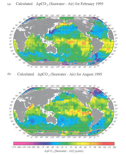
Figure 3. Distribution of climatological mean sea-air pCO difference (pCO) for the reference year 1995 representing non-El Niño conditions in February (a) and August (b). These maps are based on about 940,000 measurements of surface water pCO from 1958 through 2000. The pink lines indicate the edges of ice fields. The yellow-red colors indicate regions with a net release of CO into the atmosphere, and the blue-purple colors indicate regions with a net uptake of CO from the atmosphere. The mean monthly atmospheric pCO value in each pixel in 1995, (pCO)air, is computed using (pCO)air = (CO)air × (Pb - pH2O). (CO)air is the monthly mean atmospheric CO concentration (mole fraction of CO in dry air) from the GLOBALVIEW database (2000); Pb is the climatological mean barometric pressure at sea level from the Atlas of Surface Marine Data (1994); and the water vapor pressure, pHO, is computed using the mixed layer water temperature and salinity from the World Ocean Database (1998) of NODC/NOAA. The sea-air pCO difference values in the reference year 1995 have been computed by subtracting the mean monthly atmospheric pCO value from the mean monthly surface ocean water pCO value in each pixel.

The temperate regions of the North Pacific and Atlantic oceans take up a moderate amount of CO (blue) during the northern winter (Figure 3a) and release a moderate amount (yellow-green) during the northern summer (Figure 3b). This pattern is the result primarily of seasonal temperature changes. Similar seasonal changes are observed in the southern temperate oceans. Intense regions of CO uptake (blue-purple) are seen in the high-latitude northern ocean in summer (Figure 3b) and in the high-latitude South Atlantic and Southern oceans near Antarctica in austral summer (Figure 3a). The uptake is linked to high biological utilization of CO in thin mixed layers. As the seasons progress, vertical mixing of deep waters eliminates the uptake of CO.

These observations point out that the pCO in high-latitude oceans is governed primarily by deepwater upwelling in winter and biological uptake in spring and summer, whereas in the temperate and subtropical oceans, the pCO is governed primarily by water temperature. The seawater pCO is highest during winter in subpolar and polar waters, whereas it is highest during summer in the temperate regions. Thus the seasonal variation of pCO and therefore the shift between net uptake and release of CO in subpolar and polar regions is about 6 months out of phase with that in the temperate regions.

The pCO maps are combined with the solubility (s) in seawater and the kinetic forcing function, the gas transfer velocity (k), to produce the flux:

F = k•s•pCO                           (1)

The gas transfer velocity is controlled by near-surface turbulence in the liquid boundary layer. Laboratory studies in wind-wave tanks have shown that k is a strong but non-unique function of wind speed. The results from various wind-wave tank investigations and field studies indicate that factors such as fetch, wave direction, atmospheric boundary layer stability and bubble entrainment influence the rate of gas transfer. Also, surfactants can inhibit gas exchange through their damping effect on waves. Since effects other than wind speed have not been well quantified, the processes controlling gas transfer have been parameterized solely with wind speed, in large part because k is strongly dependent on wind, and global and regional wind-speed data are readily available.

Several of the frequently used relationships for the estimation of gas transfer velocity as a function of wind speed are shown in Figure 4 to illustrate their different dependencies. For the Liss and Merlivat (1986) relationship, the slope and intercept of the lower segment was determined from an analytical solution of transfer across a smooth boundary. For the intermediate wind regime, the middle segment was obtained from a field study in a small lake, and results from a wind-wave tank study were used for the high wind regime after applying some adjustments. This relationship is often considered the lower bound of gas transfer-wind speed relationships.

Figure 4. Graph of the different relationships that have been developed for the estimation of the gas transfer velocity, k, as a function of wind speed. The relationships were developed from wind-wave tank experiments, oceanic observations, global constraints and basic theory. The different forms of the relationships are summarized in Table 1. U is wind speed at 10 m above the sea surface.

The quadratic relationship of Wanninkhof (1992) was constructed to follow the general shape of curves derived in wind-wave tanks but adjusted so that the global mean transfer velocity corresponds with the long-term global average gas transfer velocity determined from the invasion of bomb C into the ocean. Because the bomb C is also used as a diagnostic or tuning parameter in global ocean biogeochemical circulation models, this parameterization yields internally consistent results when used with these models, making it one of the more favored parameterizations.

Using the same long-term global C constraint but basing the general shape of the curve on recent CO flux observations over the North Atlantic determined using the covariance technique, Wanninkhof and McGillis (1999) proposed a significantly stronger (cubic) dependence with wind speed. This relationship shows a weaker dependence on wind for wind speeds less than 10 ms and a significantly stronger dependence at higher wind speeds. However, the relationship is not well constrained at high wind speeds because of the large scatter in the scarce observations. Both the U and U relationships fit within the data envelope of the study, but the U relationship provides a significantly better fit. Nightingale et al. (2000) determined a gas exchange-wind speed relationship based on the results of a series of experiments utilizing deliberately injected sulfur hexafluoride (SF), He and non-volatile tracers performed in the last decade.

The global oceanic CO uptake using different wind speed/gas transfer velocity parameterizations differs by a factor of three (Table 1). The wide range of global CO fluxes for the different relationships illustrates the large range of results and assumptions that are used to produce these relationships. Aside from differences in global oceanic CO uptake, there are also significant regional differences. Figure 5 shows that the relationship of W&M-99 yields systematically lower evasion rates in the equatorial region and higher uptake rates at high latitudes compared with W-92, leading to significantly larger global CO uptake estimates.

Figure 5. Effects of the various gas transfer/wind speed relationships on the estimated air-sea exchange flux of CO in the ocean as a function of latitude. The global effects on the net air-sea flux are given in Table 1.

In addition to the non-unique dependence of gas exchange on wind speed, which causes a large spread in global air-sea CO flux estimates, there are several other factors contributing to biases in the results. Global wind-speed data obtained from shipboard observations, satellites and data assimilation techniques show significant differences on regional and global scales. Because of the non-linearity of the relationships between gas exchange and wind speed, significant biases are introduced in methods of averaging the product of gas transfer velocity and wind speed. The common approach of averaging the pCO and k separately over monthly periods, determining the flux from the product and ignoring the cross product leads to a bias that is about 0.2 to 0.8 Pg C yr lower in the global uptake estimate. This bias shows a regional variation that is dependent on the distribution and magnitude of winds. This issue has been partly rectified in some of the relationships in which a global wind-speed distribution is used to create separate relationships between gas transfer and wind speed for short-term (a day or less) and long-term (a month or more) periods. Since wind-speed distributions are regionally dependent and vary on time scales of hours, this approach is far from perfect.

The groundwork of efforts laid over the past decade and recently improved technologies make the quantification of regional and global CO fluxes a more tractable problem now. Satellites equipped with scatterometers that are used to determine wind speed offer daily global coverage. Moreover, these instruments measure sea-surface roughness that is directly related to gas transfer. This remotely sensed information, along with regional statistics of wind-speed variability on time scales shorter than a day, offers the real possibility that more accurate gas transfer velocities will be obtained. Efforts are underway to increase the coverage of pCO through more frequent measurements and data assimilation techniques, again utilizing remote sensing of parameters such as sea-surface temperature and wind speed. Better quantification of the fluxes will lead to better boundary conditions for models and improved forecasts of atmospheric CO concentrations.

Distribution of the Climatological Mean Net Sea-air CO₂ Flux

To illustrate the sensitivity of the gas transfer velocity and thus the sea-air CO flux to wind speed, we have estimated the regional and global net sea-air CO fluxes using two different formulations for the CO gas transfer coefficient across the sea-air interface: the quadratic U dependence of W-92 and the cubic U dependence of W&M-99. In addition, we have demonstrated the effects of wind-speed fields on the computed sea-air CO flux using the National Center for Environmental Prediction (NCEP)-41 mean monthly wind speed and the NCEP-1995 mean monthly wind speed distributions over 4° × 5° pixel areas.

In Table 2 the fluxes computed using the W-92 and the NCEP/National Center for Atmospheric Research (NCAR) 41-year mean wind are listed in the first row for each grouping in column one (for latitudinal bands, oceanic regions and regional flux). The column "Errors in Flux" located at the extreme right of Table 2 lists the deviations from the mean flux that have been determined by adding or subtracting one standard deviation of the wind speed (about ±2 m sec on the global average) from the mean monthly wind speed in each pixel area. These changes in wind speeds affect the regional and global flux values by about ±25%. The fluxes computed using the single year mean wind speed data for 1995 are listed in the second line in each column one grouping in the table.

The global ocean uptake estimated using the W-92 and the NCEP 41-yr mean wind speeds is –2.2 ± 0.4 Pg C yr. This is consistent with the ocean uptake flux of –2.0 ± 0.6 Pg C yr during the 1990s (Keeling et al., 1996; Battle et al., 2000) estimated from observed changes in the atmospheric CO and oxygen variations.

The wind speeds for 1995 are much lower than the 41-year mean in the northern hemisphere and higher over the Southern Ocean. Accordingly, the northern ocean uptake of CO is weaker than the climatological mean, and the Southern Ocean uptake is stronger. The global mean ocean uptake flux of –1.8 Pg C yr using the NCEP-1995 winds is about 18% below the climatological mean of –2.2 Pg C yr, but it is within the ±25% error estimated from the standard deviation of the 41-yr mean wind speed data.

When the cubic wind speed dependence (W&M-99) is used, the CO fluxes in higher latitude areas with strong winds are increased by about 50%, as are the errors associated with wind speed variability. The global ocean uptake flux computed with the 41-year mean wind speed data and the NCEP-1995 wind data is –3.7 Pg C yr and –3.0 Pg C yr respectively, an increase of about 70% over the fluxes computed from the W-92 dependence. These flux values are significantly greater than the flux based on atmospheric CO and oxygen data (Keeling et al., 1996; Battle et al., 2000). However, the relative magnitudes of CO uptake by ocean basins (shown in % in the regional flux grouping in the last four rows of Table 2) remain nearly unaffected by the choice of the wind-speed dependence of the gas transfer velocity.

The distribution of winds can also influence the calculated gas transfer velocity. This is because of the nonlinear dependence of gas exchange with wind speed; long-term average winds underestimate flux especially for strongly non-linear dependencies. To avoid this bias, the relationships are adjusted by assuming that the global average wind speed is well represented by a Rayleigh distribution function. As noted by Wanninkhof et al. (2001), this overestimates the flux. A more appropriate way to deal with the issue of wind speed variability is to use short-term winds. If the NCEP 6-hour wind products are used, the global flux computed using the W&M-99 cubic wind-speed formulation decreases from –3.7 to –3.0 Pg C yr for the NCEP 41-year winds and from –3.0 to –2.3 Pg C yr for the NCEP 1995 wind data.

The relative importance of the major ocean basins in the ocean uptake of CO may be assessed on the basis of the CO fluxes obtained from our pCO data and W-92 gas transfer velocity (Table 2 and Figure 6). The Atlantic Ocean as a whole, which has 23.5% of the global ocean area, is the region with the strongest net CO uptake (41%). The high-latitude northern North Atlantic, including the Greenland, Iceland and Norwegian seas, is responsible for a substantial amount of this CO uptake while representing only 5% of the global ocean in area. This reflects a combination of two factors: the intense summertime primary production and the low CO concentrations in subsurface waters associated with recent ventilation of North Atlantic subsurface waters. The Pacific Ocean as a whole takes up the smallest amount of CO (18% of the total) in spite of its size (49% of the total ocean area). This is because mid-latitude uptake (about 1.1 Pg C yr) is almost compensated for by the large equatorial release of about 0.7 Pg C yr. If the equatorial flux were totally eliminated, as during very strong El Niño conditions, the Pacific would take up CO to an extent comparable to the entire North and South Atlantic Ocean. The southern Indian Ocean is a region of strong uptake in spite of its small area (15% of the total). This may be attributed primarily to the cooling of tropical waters flowing southward in the western South Indian Ocean.

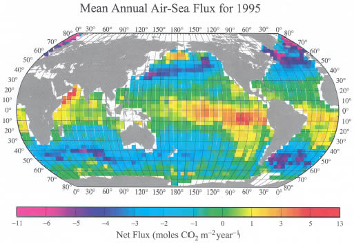
Figure 6. Distribution of the climatological mean annual sea-air CO flux (moles CO m yr) for the reference year 1995 representing non-El Niño conditions. This has been computed using the mean monthly distribution of sea-air pCO difference, the climatological NCEP 41-year mean wind speed and the wind-speed dependence of the CO gas transfer velocity of Wanninkhof (1992). The yellow-red colors indicate a region characterized by a net release of CO to the atmosphere, and the blue-purple colors indicate a region with a net uptake of CO from the atmosphere. This map yields an annual oceanic uptake flux for CO of 2.2 ± 0.4 Pg C yr.

Distribution of Anthropogenic CO₂ in the Oceans

To understand the role of the oceans as a sink for anthropogenic CO, it is important to determine the distribution of carbon species in the ocean interior and the processes affecting the transport and storage of CO taken up from the atmosphere. Figure 7 shows the typical north-south distribution of DIC in the Atlantic, Indian, and Pacific oceans prior to the introduction of anthropogenic CO. In general, DIC is about 10–15% higher in deep waters than at the surface. Concentrations are also generally lower in the Atlantic than the Indian ocean, with the highest concentrations found in the older deep waters of the North Pacific. The two basic mechanisms that control the distribution of carbon in the oceans are the solubility and biological pumps.

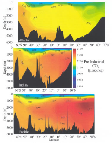
Figure 7. Zonal mean pre-industrial distributions of dissolved inorganic carbon (in units of µmol kg) along north-south transects in the Atlantic, Indian and Pacific oceans. The Pacific and Indian Ocean data are from the Global CO Survey (this study), and the Atlantic Ocean data are from Gruber (1998).

The solubility pump is driven by two interrelated factors. First, CO is more than twice as soluble in cold polar waters than in warm equatorial waters. As western surface boundary currents transport water from the tropics to the poles, the waters are cooled and absorb more CO from the atmosphere. Second, the high-latitude zones are also regions where intermediate and bottom waters are formed. As these waters cool, they become denser and sink into the ocean interior, taking with them the CO accumulated at the surface.

The primary production of marine phytoplankton transforms CO and nutrients from seawater into organic material. Although most of the CO taken up by phytoplankton is recycled near the surface, a substantial fraction, perhaps 30%, sinks into the deeper waters before being converted back into CO by marine bacteria. Only about 0.1% reaches the seafloor to be buried in the sediments. The CO that is recycled at depth is slowly transported over long distances by the largescale thermohaline circulation. DIC slowly accumulates in the deep waters as they travel from the Atlantic to the Indian and Pacific oceans. Using a 3-D global carbon model, Sarmiento et al. (1995) estimated that the natural solubility pump is responsible for about 20% of the vertical gradient in DIC; the remaining 80% originates from the biological pump.

The approaches for estimating anthropogenic CO in the oceans have taken many turns over the past decade. Siegenthaler and Sarmiento (1993) summarized early approaches for estimating the anthropogenic sink in the oceans, including ocean models of various complexity, atmospheric measurements and transport models used together with pCO measurements and estimates based on changes in oceanic C and oxygen mass balance. They noted the wide range of ocean uptake estimates (1.6–2.3 Pg C yr) and concluded that the larger uptake estimates from the models were the most reliable.

The first approaches for using measurements to isolate anthropogenic CO from the large, natural DIC signal were independently proposed by Brewer (1978) and Chen and Millero (1979). Both these approaches were based on the premise that the anthropogenic DIC concentration could be isolated from the measured DIC by subtracting the contributions of the biological pump and the physical processes, including the pre-industrial source water values and the solubility pump.

Gruber et al. (1996) improved the earlier approaches by developing the C* method. This method is based on the premise that the anthropogenic CO concentration (C^ant) can be isolated from measured DIC values (C^m) by subtracting the contribution of the biological pumps (C^bio), the DIC the waters would have in equilibrium with a preindustrial atmospheric CO concentration of 280 ppm (C^eq280), and a term that corrects for the fact that surface waters are not always in equilibrium with the atmosphere (C^diseq):

C^ant = C^m – C^bio – C^eq280 – C^diseq = C* – C^diseq.             (2)

The three terms to the right of the first equal sign make up C*, which can be explicitly calculated for each sample. The fact that C* is a quasi-conservative tracer helps remedy some of the mixing concerns arising from the earlier techniques (Sabine and Feely, 2001). The C^diseq term is evaluated over small isopycnal intervals using a water-mass age tracer such as CFCs.

We have evaluated anthropogenic CO for the Atlantic, Indian, and Pacific oceans using the C* approach. Figure 8 shows representative sections of anthropogenic CO for each of the ocean basins. Surface values range from about 45 to 60 µmol kg. The deepest penetrations are observed in areas of deep water formation, such as the North Atlantic, and intermediate water formation, such as 40–50°S. Integrated water column inventories of anthropogenic CO exceed 60 moles m in the North Atlantic (Figure 9). Areas where older waters are upwelled, like the high-latitude waters around Antarctica and Equatorial Pacific waters, show relatively shallow penetration. Consequently, anthropogenic CO inventories are all less than 40 moles m in these regions (Figure 9).

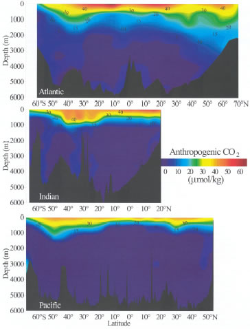
Figure 8. Zonal mean distributions of estimated anthropogenic CO concentrations (in units of µmol kg) along north-south transects in the Atlantic, Indian and Pacific oceans. The Pacific and Indian Ocean data are from the Global CO Survey (this study), and the Atlantic Ocean data are from Gruber (1998).

Figure 9. Zonal mean anthropogenic CO inventories (in units of moles m) in the Atlantic, Indian and Pacific oceans.

Data-based estimates indicate that the oceans have taken up approximately 105 ± 8 Pg C since the beginning of the industrial era. Current global carbon models generally agree with the total inventory estimates, but discrepancies still exist in the regional distribution of the anthropogenic inventories. Some of these discrepancies stem from deficiencies in the modeled circulation and water mass formation. There are also a number of assumptions in the data-based approaches regarding the use of constant stoichiometric ratios and time-invariant air-sea disequilibria that may be inadequate in some regions. These are all areas of current research. Anthropogenic estimates should continue to converge as both the models and the data-based approaches are improved with time.

Conclusions

As CO continues to increase in the atmosphere, it is important to continue the work begun with the Global Survey of CO in the Ocean. Because CO is an acid gas, the uptake of anthropogenic CO consumes carbonate ions and lowers the pH of the ocean. The carbonate ion concentration of surface seawater in equilibrium with the atmosphere will decrease by about 30% and the hydrogen ion concentration will increase by about 70% with a doubling of atmospheric CO from pre-industrial levels (280 to 560 ppm). As the carbonate ion concentration decreases, the buffering capacity of the ocean and its ability to absorb more CO from the atmosphere is diminished. Over the long term (millennial time scales) the ocean has the potential to absorb as much as 85% of the anthropogenic CO that is released into the atmosphere. Because the lifetime of fossil fuel CO in the atmosphere ranges from decades to centuries, mankind's reliance on fossil fuel for heat and energy will continue to have a significant effect on the chemistry of the earth's atmosphere and oceans and therefore on our climate for many centuries to millennia.

Plans are being formulated in several countries, including the United States, to establish a set of repeat sections to document the increasing anthropogenic inventories in the oceans. Most of these sections will follow the lines occupied during the WOCE Hydrographic Programme on which JGOFS investigators made CO survey measurements. The current synthesis effort will provide an important baseline for assessment of future changes in the carbon system. The spatially extensive information from the repeat sections, together with the temporal records from the time-series stations and the spatial and temporal records available from automated surface pCO measurements on ships of opportunity, will greatly improve our understanding of the ocean carbon system and provide better constraints on potential changes in the future.

Acknowledgements

The authors are grateful to the members of the CO Science Team and the JGOFS and WOCE investigators for making their data available for this work. We thank Lisa Dilling of the National Oceanic and Atmospheric Administration (NOAA) Office of Global Programs, Don Rice of the National Science Foundation and Mike Riches of the Department of Energy (DOE) for their efforts in coordinating this research. This work was supported by DOE and NOAA as a contribution to the U.S. JGOFS Synthesis and Modeling Project (Grant No. GC99-220) and by grants to Taro Takahashi from NSF (OPP-9506684) and NOAA (NA16GP01018). This publication was supported by the Joint Institute for the Study of the Atmosphere and Ocean (JISAO) under NOAA Cooperative Agreement #NA67RJO155, Contribution #832, and #2331 from the NOAA/Pacific Marine Environmental Laboratory. This is U.S. JGOFS Contribution Number 683.

References

Atlas of Surface Marine Data, 1994: CD-ROM NODC-56, Ocean Climate Laboratory, NOAA.

Bates, N.R., 2001: Interannual variability of oceanic CO and biogeochemical properties in the Western North Atlantic subtropical gyre. Deep-Sea Res. II, 48(8–9), 1507–1528.

Battle, M., M.L. Bender, P.P. Tans, J.W.C. White, J.T. Ellis, T. Conway and R.J. Francey, 2000: Global carbon sinks and their variability inferred from atmospheric O and C. Science, 287, 2467–2470.

Brewer, P.G., 1978: Direct observation of oceanic CO increase. Geophys. Res. Lett., 5, 997–1000.

Chen, C.T. and F.J. Millero, 1979: Gradual increase of oceanic CO. Nature, 277, 205–206.

Feely, R.A., R. Wanninkhof, T. Takahashi and P. Tans, 1999: The influence of the equatorial Pacific contribution to atmospheric CO accumulation. Nature, 398, 597–601.

GLOBALVIEW-CO: Cooperative Atmospheric Data Integration Project—Carbon Dioxide, 2000. CDROM, NOAA CMDL, Boulder, CO. Also available on Internet via anonymous FTP to ftp.cmdl.noaa.gov, Path: ccg/co2/GLOBALVIEW.

Gruber, N., J.L. Sarmiento and T.F. Stocker, 1996: An improved method for detecting anthropogenic CO in the oceans. Global Biogeochem. Cycles, 10, 809–837.

Gruber, N., 1998: Anthropogenic CO in the Atlantic Ocean. Global Biogeochem. Cycles, 12, 165–191.

Inoue, H.Y., H. Mastueda, M. Ishii, K. Fushimi, M. Hirota, I. Asanuma and Y. Takasugi, 1995: Longterm trend of the partial pressure of carbon dioxide (pCO) in surface waters of the western North Pacific 1984–1993. Tellus, 47B, 391–413.

Keeling, C.D. and T.P. Whorf, 2000: Atmospheric CO concentrations—Mauna Loa Observatory, Hawaii, http://cdiac.esd.ornl.gov/npds/npd001.html, Carbon dioxide Information and Analysis Center, Oak Ridge, TN.

Keeling, R., S.C. Piper and M. Heinmann, 1996: Global and hemispheric CO sinks deduced from changes in atmospheric O concentration. Nature, 381, 218–221.

Liss, P.S. and L. Merlivat, 1986: Air-sea gas exchange rates: Introduction and synthesis. In: The Role of Air-Sea Exchange in Geochemical Cycling. P. Buat-Menard, ed., Reidel, Boston, 113–129.

Nightingale, P.D., G. Malin, C.S. Law, A.J. Watson, P.S. Liss, M.I. Liddicoat, J. Boutin and R.C. Upstill-Goddard, 2000: In situ evaluation of air-sea gas exchange parameterizations using novel conservative and volatile tracers. Global Biogeochem. Cycles, 14, 373–387.

Sabine, C.L. and R.A. Feely, 2001: Comparison of recent Indian Ocean anthropogenic CO estimates with a historical approach. Global Biogeochem. Cycles, 15(1), 31–42.

Sarmiento, J.L., R. Murnane and C. LeQuere, 1995: Airsea CO transfer and the carbon budget of the North Atlantic. Philos. Trans. R. Soc. Lond. (B Biol. Sci.), 348, 211–219.

Siegenthaler, U. and J.L. Sarmiento, 1993: Atmospheric carbon dioxide and the ocean. Nature, 365, 119–125.

Takahashi, T., S.C. Sutherland, C. Sweeney, A. Poisson, N. Metzl, B. Tillbrook, N. Bates, R. Wanninkhof, R.A. Feely, C. Sabine, J. Olafsson and Y. Nojiri, 2002: Global sea-air CO flux based on climatological surface ocean pCO, and seasonal biological and temperature effects, Deep-Sea Res. II, 49(9–10), 1601–1623.

Wanninkhof, R., 1992: Relationship between gas exchange and wind speed over the ocean. J. Geophys. Res., 97, 7373–7381.

Wanninkhof, R. and W.M. McGillis, 1999: A cubic relationship between gas transfer and wind speed. Geophys. Res. Lett., 26, 1889–1893.

Wanninkhof, R., S. Doney, T. Takahashi and W. McGillis, 2001: The Effect of Using Time-Averaged Winds on Regional Air-Sea CO Fluxes. In: Gas Transfer at Water Surfaces. M.A. Donelan, W.M. Drennan, E.S. Saltzman and R. Wanninkhof, eds., AGU, Washington, Geophys. Mono. Ser. Vol. 127.

Return to Abstract

PMEL Outstanding Papers

PMEL Publications Search

PMEL Homepage