There is a compelling need for regional circulation models which capture both tidal and subtidal dynamics simultaneously. Here we describe a combined tidal/subtidal technique which can be used to feed global circulation model output (or data) to regional models, and its implementation in a regional model of the southeastern Bering Sea. We also describe preliminary sensitivity studies and interannual comparisons (1995 vs. 1997) based on model output.
 
 

Coastal circulation in many parts of the world is strongly influenced by tidal mixing, as well as wind- and buoyancy-driven subtidal flows. Both tidal and subtidal flows have significant impact on the biological dynamics of coastal regions. Subtidal flows interact with tides through their shared dependence on the density field; for example, fronts generated through tidal mixing on submarine banks generate subtidal flows along the front. Traditionally, coastal models have been either tidal or subtidal, but rarely have both dynamics been captured in the same simulation. One significant obstacle to the development of such combined models has been the difficulty of constructing boundary conditions which simultaneously allow the specification of tidal information, the specification of subtidal information, and the free radiation of subtidal motions generated within the regional model’s domain.

The southeastern Bering Sea (SEBS) is one such region where tidal dynamics strongly affect subtidal circulation. Here a broad shelf supports high levels of primary production and a vigorous food chain which includes large populations of groundfish and seabirds. Recent broad-scale changes in the physical and biological character of this area have been noted, especially the appearance of coccolithophore blooms in 1997 (Vance et al., 1998). As part of NOAA’s Southeast Bering Sea Carrying Capacity program (SEBSCC) we have developed a primitive equation circulation model of the SEBS shelf and basin which includes both tidal and subtidal dynamics. We are using these physical simulations to explore the relative impact of winds, tides and heat flux in different years, and to investigate how these differences affect the fate of walleye pollock (Theragra chalcogramma) spawned in different regions of the SEBS.

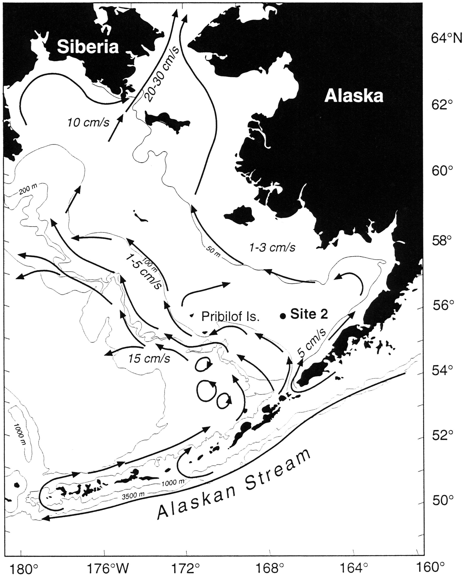
Fig. 1 Place names and schematic of mean circulation in the southeastern Bering Sea. ANSC = Aleutian North Slope Current; BSC = Bering Slope Current. Position of continuous hydrographic mooring (Site 2) is noted. Modified (with permission) from Stabeno et al. (1999).

Some of the primary physical features of the SEBS relevant to our simulations are as follows: 1. Tides and tidal mixing. The strong intensity of tidal and wind mixing, coupled with stratification by solar heating, leads to three biophysical domains on the shelf (Schumacher and Stabeno, 1998). The inner domain (0-50m depth) experiences complete mixing of the water column. The middle domain (50-100m) is characterized by a two-layer system, while the outer domain (>100m) exhibits uniform density in top and bottom layers with a gradient layer in between. 2. Flow through straits. Significant inflows to the SEBS occur through straits between the islands of the Aleutian chain, and Unimak Pass in particular. Significant outflows include Bering Strait to the north. 3. Shelf-slope exchange. Exchange between shelf and slope waters may help to fuel primary production on the shelf, but the magnitude of this exchange is very uncertain. 4. Meanders and eddies. Altimetric, SST and drifter data have revealed mesoscale features on scales from 20-200 km. 5. Ice physics and the cold pool. Each year ice formed in the Northern Bering Sea is advected south into the SEBS, where it melts. This exerts a profound effect on the heat and salt content of the shelf waters, their density stratification and their vertical mixing. A persistent pool of cold water is formed on the shelf in some years due to the influence of ice in the winter and spring. An overview of major currents in the region is illustrated in Fig. 1.
 
 

Governing Equations

Our free-surface, primitive equation circulation model is based on the S-Coordinate Rutgers University Model (Song and Haidvogel, 1994), and is implemented at 4 km horizontal resolution with 20 vertical levels. Two recent years (1995 versus 1997) are compared, based on their radically different physical and biological character and the availability of field data. Surface forcing is provided by daily NCEP winds and heat fluxes.

A substantial fraction of heat and buoyancy fluxes at the surface of the SEBS is due to ice melt. A full model of ice thermodynamics and advection was beyond the scope of this project. Instead, we rely on the observed phenomenon of ice being advected south into the SEBS and subsequently melting there (e.g. Stabeno et al., 1999). We treat ice as a forcing variable and compute daily ice melt based on ice coverage from data, and the surface temperature computed in the circulation model relative to the temperature of the ice (assumed to be -1.7 degrees C). Melt rates were calibrated using temperature data from mid-shelf mooring 2 (see Fig. 1). Ice coverage was derived from ice pack data (1/4-degree resolution) from the U.S. National Ice Center, and also by digitizing maps of ice coverage from the U. S. National Weather Service to the same grid. Computed heat and buoyancy fluxes are added at the surface of the circulation model at each model time step in place of NCEP fluxes, based on the percentage of ice cover.

Horizontal Boundary Conditions

External forcing of the regional model domain includes measured and modeled subtidal currents and five tidal components (M2, S2, N2, K1, O1) with spatially dependent amplitude and phase derived from a global implementation of the Spectral Element Ocean Model (Haidvogel et al., 1996). For the regional model itself, we employed a telescoped grid with closed walls on all sides (Fig. 2); the finely resolved (dx=dy=4 km) area lies at the center of this telescoped grid. A similar telescoped approach (but without tides) has been used successfully in regional studies of circulation and biology in the northern Gulf of Alaska (Hermann and Stabeno, 1996).

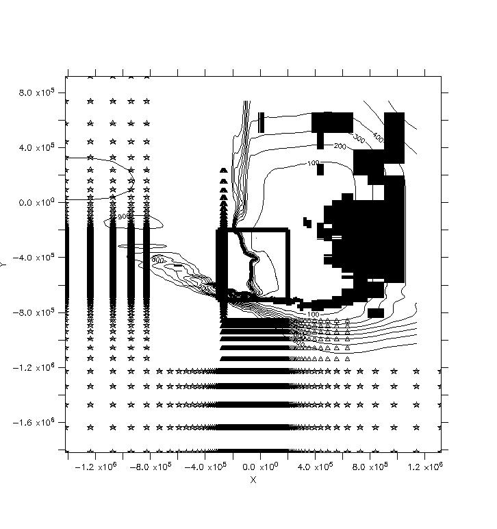
Fig. 2 Structure of the grid used by the circulation model, with bathymetry (contoured, m) and nudging bands. Land areas (Alaska and the Aleutian Islands) are indicated in black; the grid is rotated approximately 45 degrees from true north. The central box denotes the finely resolved domain with 4 km spacing. The grid is telescoped external to this area, with solid walls at the outer edge of the global domain. Stars indicate gridpoints where (fast) nudging of tidal free surface height is in effect; triangles indicate gridpoints where (slow) nudging of subtidal temperature and salinity is in effect. Small sections of the subtidal nudging band include nudging of barotropic velocity, to better assimilate the Alaskan Stream and Aleutian North Slope Current (see Fig. 1) at the boundary of the finely resolved domain.
 

To accommodate both tidal and subtidal dynamics in the present model, we employ two spatially distinct nudging bands – that is, two separate areas where the regional model assimilates tidal versus subtidal information from the larger-scale model and/or data. Tidal elevations (all five components) are assimilated in a tidal nudging band near the western and southern walls of the (telescoped) regional model domain. Temperature and salinity fields corresponding to desired subtidal inflows are assimilated along a subtidal nudging band further within the domain, but still external to the finely resolved SEBS. In each band nudging constants are linearly ramped in with weakest assimilation in effect at the inner edge, to minimize reflection and encourage absorption of internally generated signals. Subtidal barotropic velocities are also assimilated in small regions within the subtidal nudging band, to help set the value of specific boundary currents (here, the Alaskan Stream/ Alaska Coastal Current system entering from the east, and the Aleutian North Slope Flow entering from the west).

Ideally the tidal signals assimilated in the outer domain will be transmitted through areas of subtidal nudging without attenuation. In practice this transmission will depend on the value of the subtidal nudging constants for scalars and velocity, the width of the subtidal nudging band, the frequencies of the tidal signals, and the phase speeds of the tidal signals. As an estimate of attenuation, consider the one-dimensional shallow-water wave equations with nudging of tidal height and subtidal velocity:

where h is the free surface height above mean fluid depth H, u is the horizontal velocity, h^T and and u^S are the tidal height and subtidal velocity to be assimilated (from a large scale model and/or data), and a^T and a^S are the tidal and subtidal nudging constants, respectively. We seek approximate solutions for tidal motions within the subtidal nudging band. In a region where a^T = 0 and where both u^S and a^S vary slowly in space, equations (1) and (2) yield:

A characteristic equation is obtained by looking for solutions of the form:

where w may have an imaginary component. Substitution into (4) yields

If the nudging coefficient a^S is sufficiently small and the tidal frequency w^T (= kc, with units of radians per sec) is significantly large, then

Under these circumstances the solution for an incident tidal signal in the subtidal nudging band can be approximated as

Now, integrating a tidal characteristic (kx-w^Tt) across a subtidal nudging band of width dx, the fractional attenuation of tidal amplitude due to passage through that band is

For typical values in our model (dx = 2 x 10⁴m, c = 100 ms^-1 and a^S = 10^-5 s^-1), A is negligible. Indeed, even if subtidal nudging occupied the entire finely resolved region (dx = 4.4 x 10⁵ m), the value of A would be less than 0.1. Hence, barring substantial reflection of the tidal signal at the edge of the subtidal nudging band, we will have clear transmission of the tidal signal into (and back out of) the model interior.
 
 

Our model reproduces many of the major features in the SEBS; in particular, a sluggish circulation on the inner shelf, a vigorous northwestward alongshelf flow at the shelf-break, northwestward flow along the 100 meter isobath, anticyclonic flows around the Pribilof Islands (partly the result of tidal residual currents), and colder temperatures on the shelf than in the deep basin (Fig. 3). A large degree of mesoscale eddy activity (typically ~50 km diameter) is produced, with free surface height signatures (~5 cm) similar to those observed in altimetric data.

Initial runs of the model did not attempt a specific phasing of the tidal components relative to a particular year (but did include phase information in space). It has been suggested that the phasing of the tides relative to one another in time can have important effects on the seasonal pattern of mixing, and should itself exhibit interannual variability. That is, in some years the interactions of the many tidal components will lead to especially large tidal velocities, and hence more mixing in particular months or even on specific days or times of day. However, comparative runs for one month exhibited little difference between a run with arbitrarily chosen tidal phases, versus one with tides phased specifically for year 1995.

Simulations for 1995 versus 1997 exhibit significant differences in both velocity and temperature fields (compare Figs. 3 and 4). First, 1997 is much warmer than 1995, due in part to greater penetration of ice in 1995. Second, mesoscale eddy activity is much greater in 1995 than 1997. To demonstrate how this enhanced eddy activity might affect spawned walleye pollock in the Bering Sea, we conducted a simple float tracking experiment using depth-averaged velocities (including tides). Floats released near the shelf break in 1995 exhibited a greater tendency to wander off into the deep basin, relative to their equivalents in 1997.

In significant portions of the SEBS the tidal velocities account for greater than 95% of the Total Kinetic Energy in current meter records. One might expect that vertical mixing would be uniformly strong in regions of high tidal energy. However, a rendering of instantaneous vertical viscosity computed from the model suggested that this is not the case; highest values were instead produced along the 100m isobath (where strong subtidal flows were generated) and along the shelf break (where both tidal and subtidal velocities are strong). Apparently the subtidal velocities contribute strongly to the overall mixing pattern.
 

Fig. 3. Subtidal (i.e. low-pass filtered) current vectors (m s^-1) and surface temperature (shaded, degrees C) from model output in the finely resolved domain (see Fig. 1) for DOY 94 1995. Model bathymetry is contoured (meters). Only every third vector is plotted in this figure; full grid spacing is 4 km. Horizontal distances are indicated in meters. The position of mooring 3 ("S3") is noted. The Pribilof Islands appear as two black dots in upper half of the figure.
 
 

Fig. 4. Model results as in Fig. 3, for DOY 94 1997.

We have compared depth-time profiles from the model with equivalent profiles from moored thermistor chains at two cross-shelf locations (60 and 120m depths, respectively). In both data
(not shown; see Stabeno et al., 1999) and model (Fig. 5), a significantly warmer water column is observed in 1997 than in 1995. Also, in both data and model the profiles at the deeper location are significantly warmer than those at the shallower site. Some specific daily events seen in the data were reproduced by the model as well. Planned studies will use this physical model output to drive spatially explicit models of walleye pollock in the Bering Sea, to help assess the impact of physical factors on their observed interannual variability.

Fig. 5 Time-depth series of simulated temperature at two mooring locations (Stn 2 at 60 m depth, Stn 3 at 120 m depth) for years 1995 and 1997. Positions of these two moorings are noted in Figs. 1 and 3, respectively.
 
 

Our combined tidal/subtidal boundary technique appears to function effectively in the Southeastern Bering Sea, a region with strong tidal and subtidal dynamics. The inclusion of both dynamics allows a proper interaction between tidal mixing and subtidal currents set by the density field. These interactions play a significant role in both physical and biological dynamics, and permit a more realistic assessment of interannual variability in the SEBS.

Haidvogel, D.B., E. Curchitser, M. Iskandarani, R. Hughes and M. Taylor. 1997. Global modeling of the ocean and atmosphere using the spectral element method. Atmosphere-Ocean 35: 505-531.

Hermann, A. J. and P. J. Stabeno. 1996. An eddy resolving model of circulation on the western Gulf of Alaska shelf. I. Model development and sensitivity analyses. J. Geophys. Res. 101: 1129-1149.

Schumacher, J.D., and P.J. Stabeno, 1998: The continental shelf of the Bering Sea. The Sea, Vol. VII: 789-822.

Song, Y. and D. B. Haidvogel. 1994. A semi-implicit ocean circulation model using a generalized topography-following coordinate system. J. Comput. Res. 115: 228-244.

Stabeno, P. J. , N. A. Bond, N. B. Kachel, S. A. Salo, and J. D. Schumacher. 1999. On the temporal variability of the physical environment over the Southeastern Bering Sea. Fish. Oceanogr., in press.

Vance, T.C., C. Baier, R.D. Brodeur, K. Coyle, M.B. Decker, T. Wyllie-Echeverria, G. Hunt, J.M. Napp, J.D. Schumacher, P.J. Stabeno, D. Stockwell, C. Tynan, T.E. Whitledge

and S. Zeeman, 1998: Union Ecosystem Anomalies in the Eastern Bering Sea: Including Blooms, Birds and Other Biota. EOS, Trans. Am Geophys. Vol. 79(10): 121-126.