Authors:
A.J. Hermann (University of Washington, Seattle)
D.B. Haidvogel (Rutgers University)
E.L. Dobbins (University of Washington, Seattle)
P.J. Stabeno (NOAA/Pacific Marine Environmental Lab, Seattle)
PMEL contribution number 2174
ABSTRACT
In order to assess the impact of interannual-to-decadal
changes in circulation and hydrography on lower trophic level dynamics
in the Coastal Gulf of Alaska (CGOA), we are developing a suite of physical
and biological models as part of the West Coast US GLOBEC program. These
include a global circulation model, a regional circulation model, a lower
trophic level (NPZ) model and an individual-based salmon model. Our global
circulation model consists of the Spectral Element Ocean Model (SEOM) implemented
in layered, primitive equation form. Our regional physical model consists
of the S-Coordinate Rutgers University Model (SCRUM) executed with a ~22km
resolution in the CGOA and driven by runoff, heat flux and wind stresses
appropriate to years 1976, 1995 and 1997. As presently structured our models
develop appropriate boundary currents (the Alaskan Stream and the Alaska
Coastal Current), and also spin up large (~200km) eddy features which appear
to play a significant role in cross-shelf exchange. Model-generated seasonal
patterns and eddy structures are consistent with recent and historical
data (hydrograhic, drifter track, SSH, and SST). As part of our model validation
for GLOBEC, we explore: 1) interannual differences in the broad regional
circulation and temperature; 2) Eulerian and Lagrangian aspects of a large
eddy feature near Sitka, Alaska; 3) the impacts of driving the regional
model boundary with data from the global circulation model, and how that
result compares with regional velocities from the global model itself.
Background
Interannual to interdecadal changes in the circulation of the Gulf of
Alaska are expected to exert considerable influence on recruitment of salmon
and other nekton in the Gulf (e.g. Hare and Francis 1995). As part of the
Northeast Pacific Global Ecosystems Dynamics Program (GLOBEC) we are developing
a primitive equation model of the Gulf of Alaska which includes both tidal
and subtidal dynamics, to help assess the physical sources of observed
biological variability.
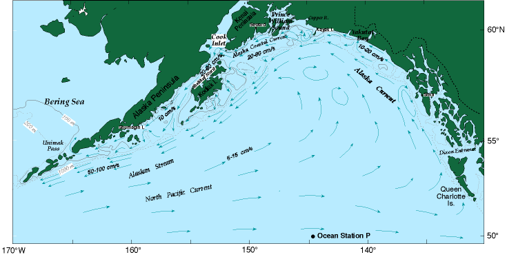
The Gulf of Alaska contains two major current systems: the Alaskan Current (AC)-Alaskan Stream (AS) system of the deep basin and shelf break, and the Alaska Coastal Current (ACC) (Fig1). The AC-AS system is part of a subarctic gyre and is forced to a large degree by wintertime cyclonic winds in the northeastern Pacific. This gyre is much broader in the eastern than in the western part of the GOA, where it forms the narrow, swift AS constrained by a steep continental rise which parallels the Aleutian Island chain. The annual mean flow of the AS is approximately 107 m3 s-1 above 500 m depth (Reed, 1984). It is generally steady on seasonal scales (despite the seasonal variation in local winds), but varies on the interannual and decadal scale (Reed, 1984; Musgrave et al., 1992; Lagerloef 1995). In AVHRR imagery, the AS typically shows up as a warm band of SST along the shelf break in the northern Gulf (Royer 1983). Chelton and Davis (1982) first suggested that the Alaska and California Current systems fluctuated out of phase on interannual time scales, both being fed by the West Wind Drift. Altimetric, SST and hydrographic data support the existence of interannual and interdecadal variability in both systems. Altimetric data analyzed by Strub (1999) suggest a possible mechanism for exhange between the gyres, that is, a possible northern coastal source for some of the waters forming the California Current.
Fig. 1. Overview of circulation in the Gulf of Alaska.
The ACC is driven by a widely distributed source of freshwater and by
local, downwelling-favorable winds (Schumacher et al., 1990; Royer 1981).
Continuity of this current in the northern and western Gulf has been established
(Stabeno et al., 1994). Large precipitation around the Gulf results from
lifting of moist marine air over the coastal mountain range; hence rivers
and streams distributed around the Gulf of Alaska provide strong buoyancy
forcing. The Copper River, at the head of the GOA, is an especially powerful
source. The riverine input is greatest in October and smallest in March
(Royer, 1982), while downwelling-favorable winds peak in January for the
northern Gulf (Royer, 1983). Moored current meter records, in conjunction
with geostrophic calculations from CTD casts, have indicated that the mean
flux of the ACC through Shelikof Strait in the spring is ~0.6 x 10⁶
m3 s-1 (Reed and Schumacher, 1989; Reed and Bograd,
1995).
Spatial variability in the AC-AS has been observed at intermediate (~200
km) scale, with some preferred sites of formation. In particular, Tabata
(1982) noted the intermittent presence of a large eddy feature centered
off Sitka, Alaska (the "Sitka eddy"). Other large-scale meanders of the
AS have also been observed along the length of the AS, most notably in
SST imagery analyzed by Thompson and Gower (1998).
Methods
1. The Global Model
A large-scale context for our regional studies is provided by simulations
with the Spectral Element Ocean Model of Haidvogel et al. (1999). SEOM
has been developed for the purpose of high-resolution basin-scale modeling
on unstructured global grids (Iskandarani et al., 1995). The governing
equations are the 3-D, Reynolds-averaged Navier-Stokes equations with Boussinesq
and hydrostatic assumptions. Subgridscale mixing is parameterized using
spatially dependent lateral mixing in the horizontal. The resulting class
of large-scale circulation models has several significant virtues over
those using more traditional approaches, including complete geometric flexibility,
regionally selective horizontal resolution, and the ability to avoid open
boundary conditions by use of global grid refinement.
The spectral element circulation model has now been applied in its reduced
gravity form to a variety of test problems and global oceanic/atmospheric
applications (Fig. 2). When applied to a now standard suite of shallow
water test problems on the sphere, the SEOM model is shown to be highly
competitive with other numerical models, including those based on spherical
harmonic methods (Taylor et al., 1996). Oceanic applications on global,
non-uniform grids show that these favorable properties are maintained in
the presence of continental geometry and highly unstructured elemental
meshes (Haidvogel et al., 1996).
Here, SEOM has been implemented on a global grid in layered form (5 layers). It has been spun up with 5 years of a repeating cycle of NCEP winds, corresponding to the period of NCSAT wind availability. A related study compares dynamics of the model subject to the (finer-scale) NSCAT winds, relative to NCEP (ref?).
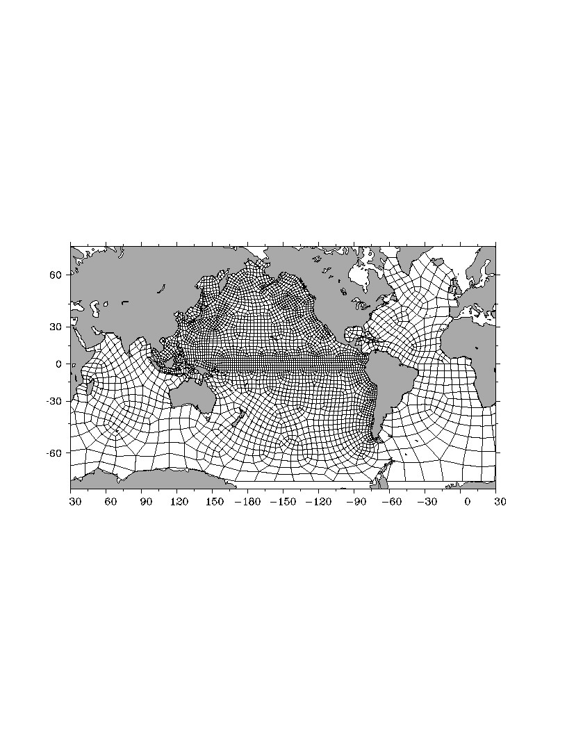
Fig. 2. Layout of quadrilateral elements for our layered implementation
of the Spectral Element Ocean Model (SEOM). Structure within each quadrilateral
is represented with a polynomial basis set.
2. The Regional Model
To capture regional circulation in the CGOA, we employed the S-Coordinate Rutgers University model (SCRUM) of Song and Haidvogel (1992). This free surface, primitive equation model uses curvilinear-orthogonal coordinates in the horizontal, while the stretched, bottom-following "s-coordinate" allows for flexible spacing of vertical grid points (Song and Haidvogel, 1992). The latter feature is especially useful in resolving boundary layers at the top of the water column (important for wind mixing) and near the bottom (important for tidal mixing). Initial experiments with a coast-following versus rectilinear coordinate system established the latter as the more economical choice for the highly curved CGOA coastline. Ultimately we implemented the model on a rectilinear telescoped grid, oriented at 45 degrees to true north. In SCRUM, land areas are "masked out" after the calculation of each timestep, but still entail some computational overhead. Our rotated grid is designed to efficiently cover coastal and basin areas of the GOA, while minimizing coverage of land areas to enhance computational efficiency.
A telescoped horizontal grid was employed to further reduce computational
overhead associated with horizontal boundary conditions. The grid has 145
x 113 horizontal gridpoints with 17 telescoped gridpoints on the southern
and western boundaries (Fig. 2). The finely resolved area of the model
domain reaches from the northeast corner to Queen Charlotte Island in the
south and Unimak Pass in the west. The telescoped region continues to the
south end of Vancouver Island, and to Amukta Pass in the west. Grid resolution
varies from 22 km in the finely resolved area, to 200 km near the western
and southern walls. As described in a subsequent section, the telescoped
regions here serve primarily to recirculate flows into and out of the area
of interest.
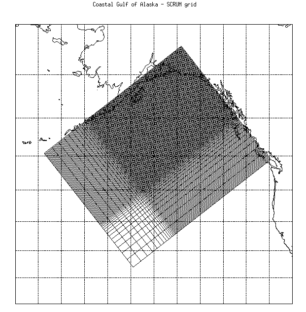
Fig. 3. Layout of the telescoped rectilinear grid for our regional implementation
of the S-Coordinate Rutgers University Model (SCRUM).
To allow proper resolution of top and bottom boundary layers, we employed 20 vertical levels. We utilized the s-coordinate feature of SCRUM to achieve quasi-uniform spacing near the surface, with limits of ?X m in the shallowest areas and ?Ym in the deepest areas.
Our CGOA implementation of SCRUM is forced by winds, coastal runoff
and atmospheric heat flux. Details of the forcing, bathymetry, and boundary
conditions are given in the following sections.
Bathymetry
Model bathymetry was interpolated from a specially developed 5-minute
bathymetric map of the CGOA, based on ETOPO5 and other sources. While ETOPO5
has the advantage of broad coverage, it is well known to be inaccuarate
in many coastal areas. More detailed and accurate bathymetric data to improve
ETOPO5 was obtained from two different sources: 1) Nearshore data from
the National Ocean Service (NOS) Hydrographic Data Base, error checked
and gridded to 30 seconds by National Geophysical Data Center (NGDC) and
distributed as the TerrainBase data collection. These data are focused
on specific coastal areas such as Cook Inlet in the CGOA. 2) Offshore data
from Smith and Sandwell (1997), who collected and verified coastline and
marine ship track data from many sources, and distributed that data as
part of their 2 minute measured and estimated digital topographic map.
Though their estimated bathymetry (based partly on gravity anomalies) contains
too much noise to be useful on the continental shelf, the measured bathymetry
was easily extracted and used to improve ETOPO5 values offshore. A complete
collection of descriptions of available bathymetry and topographic data
sets has been compiled by Robert A. Kamphaus (ref?).
Data from these two detailed sources were combined and interpolated
to a 5-minute grid using Global Mapping Tools (GMT). To reduce computation
effort, the interpolations were done for 10 deg. by 10 deg. areas that
overlap by .25 deg. The interpolated grid points match those of ETOPO5
so that when they were combined, ETOPO5 seamlessly supplies data in areas
where the detailed bathymetry data set is lacking (the Bering Sea, for
example).
The final data set is particularly accurate in areas of high data resolution,
such as along the shelf break. It constitutes a major improvement over
ETOPO5, especially in shallow shelf areas such as the Trinity Banks southwest
of Kodiak Island. After interoplation to the SCRUM grid, bathymetry was
filtered with ?X passes of a Shapiro filter, for numerical stability of
the simulation (Fig. 3). Even after filtering, the result is considerably
more accurate than any bathymetry obtainable with ETOPO5 alone.
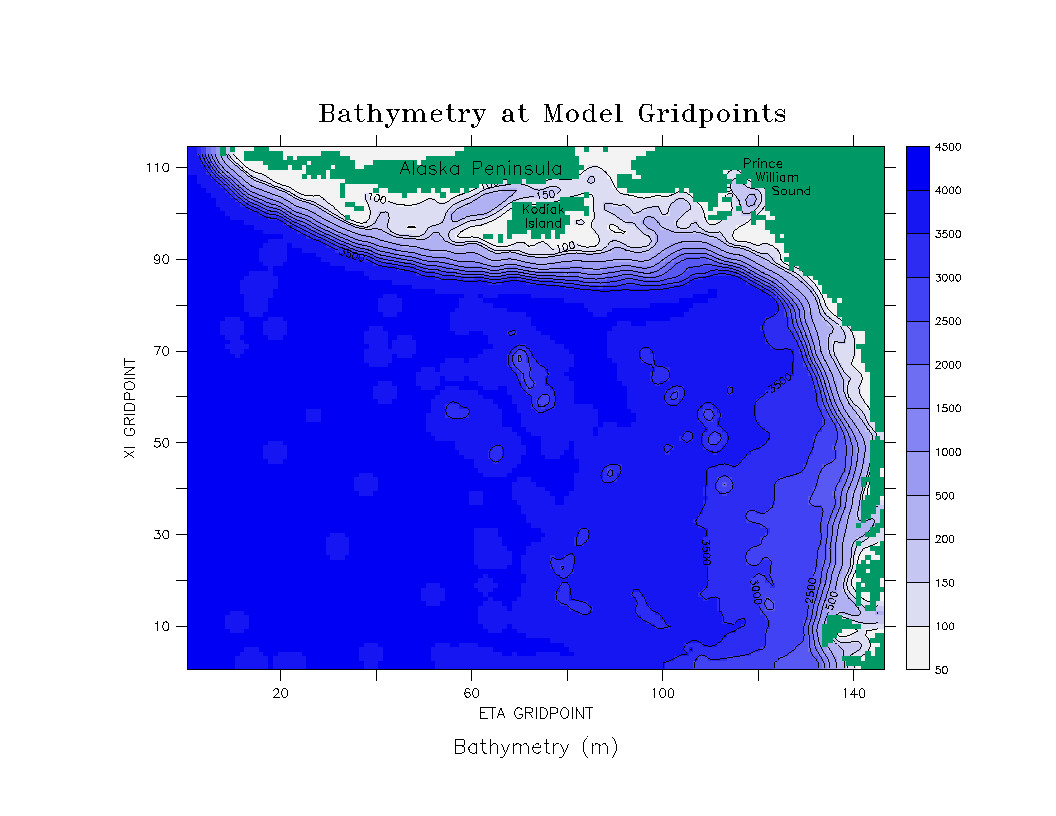
Fig. 4. Smoothed bathymetry used for the regional model simulations.
Heat Flux and Wind Stress
Both wind and heat flux contribute substantially to the near-surface
dynamics of the CGOA. Suitable values of wind and heat flux in specific
years were obtained from the NCEP/NCAR Global Reanalysis Project. NCEP
products include a global data set of atmospheric variables, obtained by
combining a global spectral model with historical data. Their model has
been run for the years 1958-present, and the output is available online.
Resolution of these data is roughly 2 degrees. Temporal resolution is 6
hours, but we have chosen to use daily averages as input to our regional
circulation model.
Daily average NCEP values for latent and sensible heat net flux, and
net longwave and shortwave radiation were summed to provide total heat
flux from the ocean. Daily average U-wind and V-wind at 10m height above
the ocean surface were converted to wind stress using the simple formula:
tao = Cd * U10 * |U10|
where U10 is the vector of wind speed in m/s and Cd = .0012 .
Freshwater Input
Freshwater from distributed sources is a major source of buoyancy to the CGOA. Time series of "line-source" freshwater input are shown in Fig. 4 for 1995. These monthly values of integrated freshwater runoff along segments of the coastline were derived from snowpack, precipitation and temperature data by Royer (1982 and pers. comm.). The data represent runoff from areas seaward of the coastal mountain range. The Southeast Coast region begins at the southern border of Alaska and extends northward to a location between Glacier Bay and Yakutat Bay. The Southcoast extends northward from there to include the southern side of the Kenai Penisula. These regions are roughly equivalent to 130W-141W and 141W-152W longitude.
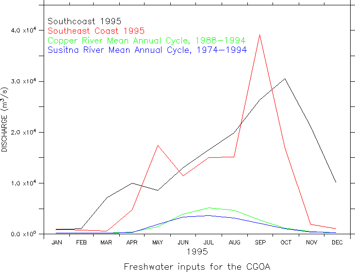
Fig. 5. Freshwater runoff for 1995, illlustrating seasonal pattern along the southeastern coast of the GOA (south of Prince William Sound: "Southeast Coast"), the southern coast of the GOA (west of Prince William Sound; "Southcoast"). Average seasonal pattern of discharge for the Copper and Susitna Rivers is also shown.
These line-source estimates were supplemented by river discharge data
for significant inland areas draining into the CGOA. The river discharge
data were obtained from USGS sources. The Susitna and Copper Rivers were
among the few rivers that were gauged, and there were not many years of
data for either. Therefore, a monthly climatology was computed with all
the available data, and this is used for every model year. Note how little
discharge is provided by these large rivers, as compared to the line-source
discharge.
Mixing
Vertical mixing is parameterized as a function of local shear and stability,
using Mellor-Yamada level 2.0 closure. Horizontal mixing of both scalars
and momentum is calculated with a biharmonic operator, and scaled by the
local grid spacing as described in Hermann and Stabeno (1996). Mixing is
computed along geopotential surfaces, rather than along sigma surfaces,
as described in ?(SCRUM ref manual?)
Horizontal Boundary conditions
The philosophy of our approach to regional is similar to that of Hermann
and Stabeno (1996), as follows. True open boundary conditions are difficult
to achieve in eddy resolving models, and especially so if tidal motions
must be permitted simultaneously. Open boundaries are notoriously unstable
to vigorous mesoscale signals; it has been suggested that the problem is
mathematically ill-posed (ref). One sensible approach is to avoid open
boundaries entirely through the use of a telescoped grid and a simple closed
box (Fig x). Within this box, adjacent to the finely resolved area of interest,
are placed bands where flow and scalar values are nudged towards desired
values, but not so strongly as to prevent the escape of any out-going,
internally-generated mesoscale signals. The desired boundary values may
be based on data or an externally run large scale model, or some combination
of the two. The area between nudging bands and the solid wall is intended
to function as a free recirculation zone, satisfying continuity and possibly
absorbing any mesoscale features which escape from the interior.
When both tidal and subtidal forcing is desired, a useful approach is
to separately apply the tidal signal on sea surface elevation in a nudging
band adjacent to the solid wall. If nudging constants for the subtidal
nudging band are chosen properly, this signal will pass cleanly through
that band without interference. In the present work, we will show only
results from the subtidally-nudged model. Future work will add simultaneous
tidal forcing, as has been accomplished for the Bering Sea (Moscow ext
abs ref)
Float Tracking
Ultimately this physical model will feed information to a three-dimensional
lower trophic level (NPZ) model, and an individual-based model of juvenile
salmon (Fig. 1). The NPZ model is designed to include preferred prey of
juvenile salmon (e.g. euphausiids), and is currently running in one-dimensional
(depth-time) form. As an intermediate step on the path to fully coupled
models, we are tracking representative fish (here, passive numerical floats)
using surface currents generated by the regional physical model. A population
of sockeye salmon juveniles has historically been observed in July just
northwest of the Queen Charlotte Islands; hence our floats are seeded in
north-south lines at 0,100,200,300 and 400km from the coast just north
of the tip of that island. Subsequent tracks are strongly influenced by
the Sitka Eddy, as described in the results.
Model experiments
We have set up several model experiments to test features of the coupling scheme and performance of the regional model. The experiments conducted are as follows:
1) Run of the global model. The global model is spun up with 5 years of a repeating cycle of daily NCEP winds, spanning the period of NCSAT wind availability (Aug 1996-July 1997). Resulting depth-integrated velocities were low-pass filtered and stored on a daily basis, for use by the regional model.
2) Free runs of regional model. We spin up the regional model from a state of rest, starting on January 15 of each simulated year. T and S fields are initialized with Levitus climatology for January, and driven with winds (NCEP 2 degree daily averages for that year), heat fluxes (NCEP 2 degree daily averages for that year) and runoff (Royer's monthly averages for that year plus river monthly climatologies). Runs were executed for calendar years 1976, 1995 and 1997.
3) Assimilating runs of the regional model. Here we utilize monthly climatologies (Levitus) for T and S, and daily barotropic velocities from the global model, as candidate fields to be assimilated by the regional model. Wind and coastal buoyancy forcing is applied as in the free run cases, appropriate to the period August-December 1996.
i) In the first assimilation experiment, the regional model is nudged for five model days with daily barotropic velocities (from SEOM), and monthly T,S fields (from Levitus climatology). A uniform nudging coefficient is applied in the finely resolved domain, and ramped to zero approaching the outer edges of the (telescoped) domain. This pattern of assimilation allows the interior to assume the SEOM velocity values, without forcing any flows through the solid walls. Subsequent to the five-day spinup, the model is nudged only in the telescoped domain, with nudging coefficient values ramped to zero at the edge of the finely resolved domain (Fig. xx). The initial spinup everywhere with SEOM provides the essential broad patterns of the flow field, including some larger eddies. Subsequently the regional model is free to develop finer-scale circulation in its interior, under the influence of local wind and buoyancy forcing and with the SEOM velocities and Levitus T,S applied as a horizontal boundary condition.
ii) In the second assimilation experiment, the model is spin up as in
case i). Subsequently, however, we remove all influence of the SEOM velocities,
and assimilate only the climatological T,S as a horizontal boundary condition.
By contrasting runs ii) and i), we clarify the influence of global barotropic
velocities on the interior regional solution.
Results
1) Global model results
Here we present barotropic velocities and free surface height fields from SEOM on a regular lat-long grid, for mid-July and early November (Fig xx). Coastal and shelf-break currents are evident, as are meanders and eddies in the deep basin. A significant portion of the shelf-break current in the northwestern GOA (the Alaskan Stream) appears to come from the deep basin in these simulations, in addition to shelf-break currents upstream. In early November, a spatially continuous flow proceeds westward (counterclockwise) around the GOA. Results for mid-July exhibit a significant reversal of that near-coastal flow in the eastern GOA. Seasonal weakening/reveral of the coastal currents in the eastern GOA has been noted by Royer (ref) and appears in the analyses of seasonal altimetric patterns of Strub (this volume).
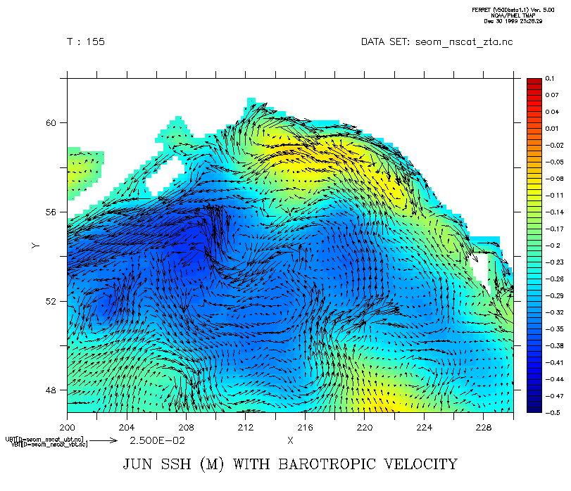
Fig 7. Global model SSH (shaded, m) and barotropic velocity (m/s) for
DOY 155.
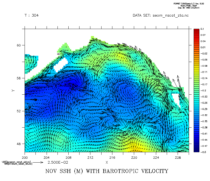
Fig 7. Global model SSH (shaded, m) and barotropic velocity (m/s) for
DOY 304.
2) Regional model free run results.
Regional model results reproduce many of the major observed features
in the CGOA. Here we examine 130-day runs initialized with Levitus climatological
January T and S and driven with winds, heat flux and runoff appropriate
to 1976, 1995, and 1997, respectively. All runs exhibit a prominent AC-AS
system and a weaker ACC. A weak ACC is appropriate for this time of year,
as buoyancy fluxes are at their seasonal minimum). An
intense and rapidly evolving eddy field is produced at the shelf-break,
with 200km as the dominant spatial scale. The train of eddies generated
around the Gulf is similar to that seen in the AVHRR imagery of Thompson
and Gower (1998). A tongue of warm water penetrates west along the shelf
break as has been noted in the SST images and in hydrographic data. A comparison
of the simulations for 1995 versus 1997 reveals warmer temperatures in
1997, but a similar degree of large eddy activity in each case. Representative
results are shown for late March 1997 and 1995 in Fig. 3.
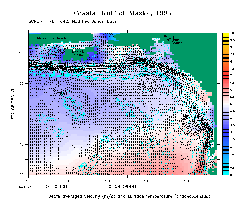
Fig. 8. Regional model SST (shaded, degrees C) and barotropic velocity
(m/s) for DOY 64.5 1995.
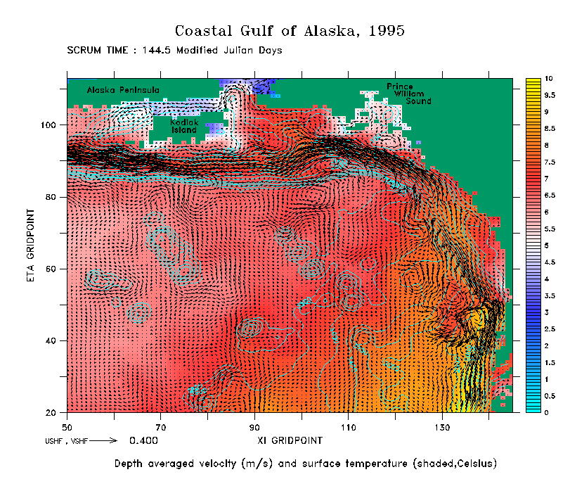
Fig 9. Regional model SST (shaded, degrees C) and barotropic velocity
(m/s) for DOY 144.5 1995.
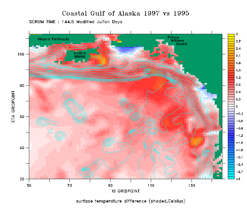
Fig 10. Difference in regional model SST for 1997 vs 1995 at DOY 144.5.
Note pervasive warming, especially at the location of the Sitka eddy.
Mesoscale circulations are observed in model output, locked to prominent
seamounts in the deep basin. Animated results exhibit a clockwise propogation
of disturbances around these seamounts.
Eddies in the GOA with ~200km scale have
been measured with sea surface height (TOPEX), sea surface temperature
(AVHRR), and hydrographic (T, S, O2) data. TOPEX data in particular
has indicated lifespans of months to years (Josef's paper).
They typically drift at < 2 cm/s, are predominantly anticyclonic, are
more commonly observed in spring. Other modeling studies have suggested
that such eddies near the shelf break are possibly intensified by ENSO
warm events (Melsom et al. 1999). During the first week of March, 1995,
the model generates eddies whose locations roughly correspond to those
which have been observed by AVHRR on this date (Figures 7 and 8). However,
the temperature signals are less evident than the velocity signals.
In our model, 200-km scale eddy activity is most prominent in the vicinity of Sitka (Fig. 4), at a location slightly north of the traditionally reported "Sitka eddy" (refs). The Sitka eddy has been reported in other studies as topographically generated, and has average surface currents of 15 cm/s, with a maximum of 110 cm/s as measured by drifters. Our model-generated surface drifter tracks in this area (Fig. 5) compare favorably with observed drifter tracks, but do tend to exhibit weaker velocities than observed. Specifically, the drifters in Figure 5 transit the Sitka eddy in about 11 days, while the model's drifters (Figure 6) require about 30 days to complete one circuit.
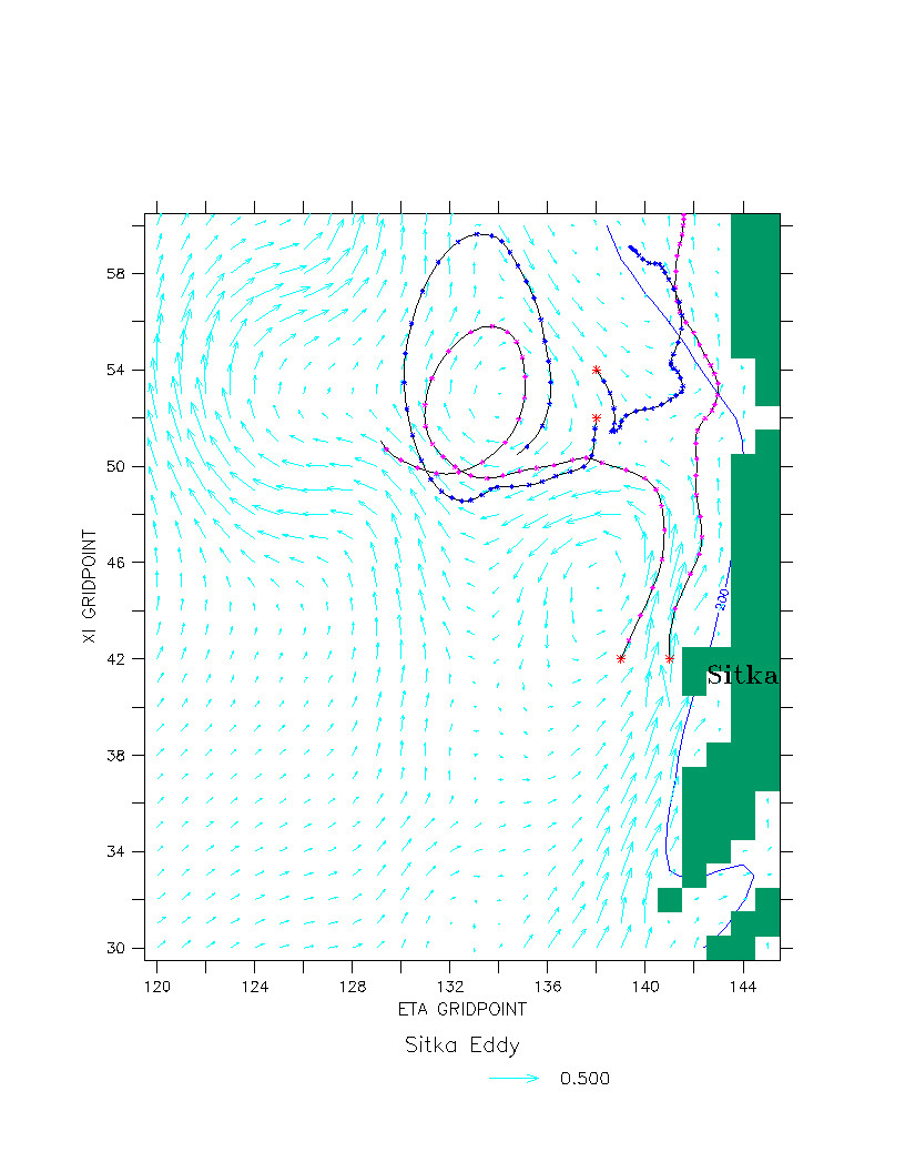
Fig. 11. Regional model float tracking experiment using surface velocities
in the vicinity of Sitka, AK.
Our regional model results for 1976 include a persistent Sitka eddy
moving slowly offshore from Spring to Fall (Fig. xx). This behavior has
been observed in the layered model studies of Melsom et al. (1999).
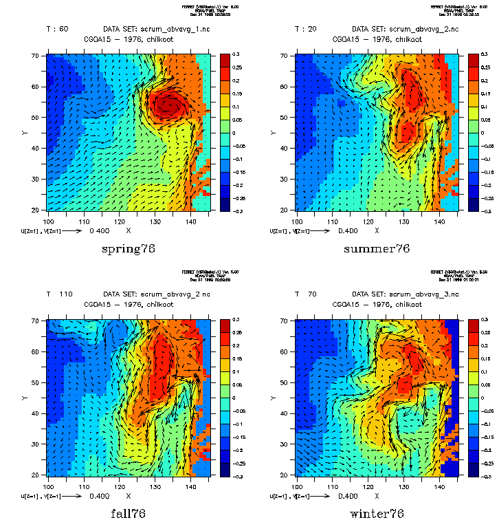
Fig. 12. Regional model results for 1976: SSH relative to areal mean (shaded, m) and surface velocities (m/s) in the vicinity of Sitka, AK for March (spring), June (summer), September (fall) and December (winter). Note the gradual migration of the "Sitka eddy" offshore from Spring through Winter 1976
Numerical drifter tracks for July-Dec 1976 (Fig. 13 a-e) underscore
the significance of the large eddy activity, and the Sitka eddy in particular,
to salmon dynamics in the Gulf. Half of the drifters released near the
coast (Fig. 13a) become trapped in the Sitka eddy, with penetration further
north only for tracks very close to the coastline. Drifters released 100km
offshore (Fig. 13b) exhibit similar entrapment in the eddy feature. At
200km (Fig. 13c) offshore most of the drifters move around the western
rim of the eddies; these either merge into the Alaskan Stream, traveling
far to the west, or run aground between Sitka and Prince William Sound
due to downwelling circulation (Fig. 5). Releases at 300 and 400km offshore
(Fig. 13d,e) typically run aground somewhere between Yakutat Bay (east
of Prince William Sound) and Cook Inlet (east of Kodiak Island). These
early results help demonstrate the importance of accurate spatial tracking
of individual fish, including the influence of mesoscale eddies.
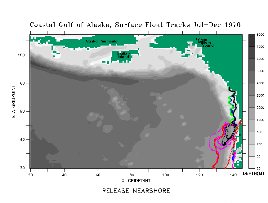
Fig 13. a) Regional model float tracking experiments using surface velocities.
Floats are released nearshore to the south of Sitka AK (indicated by asterisk
in figure), and subsequently tracked for July-Dec 1976.
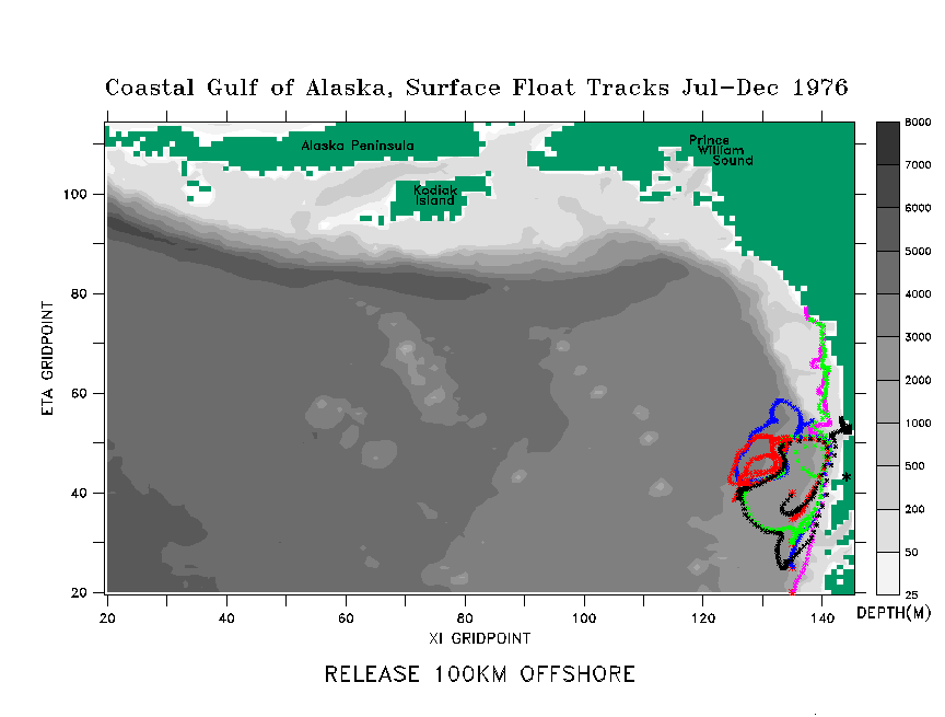
Fig 13. b) Float tracks subsequent to release 100km offshore.
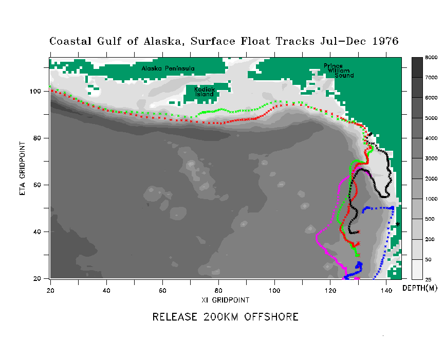
Fig 13. c) Float tracks subsequent to release 200km offshore.
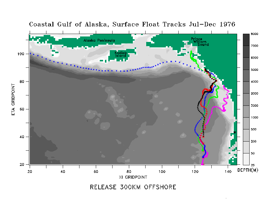
Fig 13. d) Float tracks subsequent to release 300km offshore.
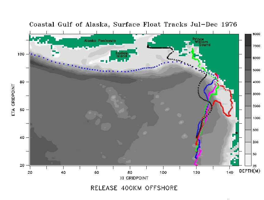
Fig 13. e) Float tracks subsequent to release 400km offshore.
3) Assimilating run results
Here we compare: 1) the global model (SEOM) barotropic velocity results; 2) a reional model run assimilating both global barotropic velocities (from SEOM output) and T,S climatology; 3) a regional model run assimiliating T,S climatology only. Results of each case are presented on the grid used by the regional model (in the case of the global model, results from the unstructured grid were interpolated onto this regular grid).
Each of the regional model simulations was begun from a state of rest on August 1, initialized with T,S climatology appropriate to that date. After a 90 spinup, substantial differences have emerged among the three cases. The velocities associated with the SEOM fields have penetrated far along the coastal waveguide and, to a lesser degree, into the interior of the basin. This is consistent with the fast propagation of coastally trapped signals.
First, consider the global model results for early Novemeber 1996. As noted in previous figures, the velocities in the global model are generally weaker than those in the regional model. In particular, the Alaskan Stream is less well developed than in the regional model.
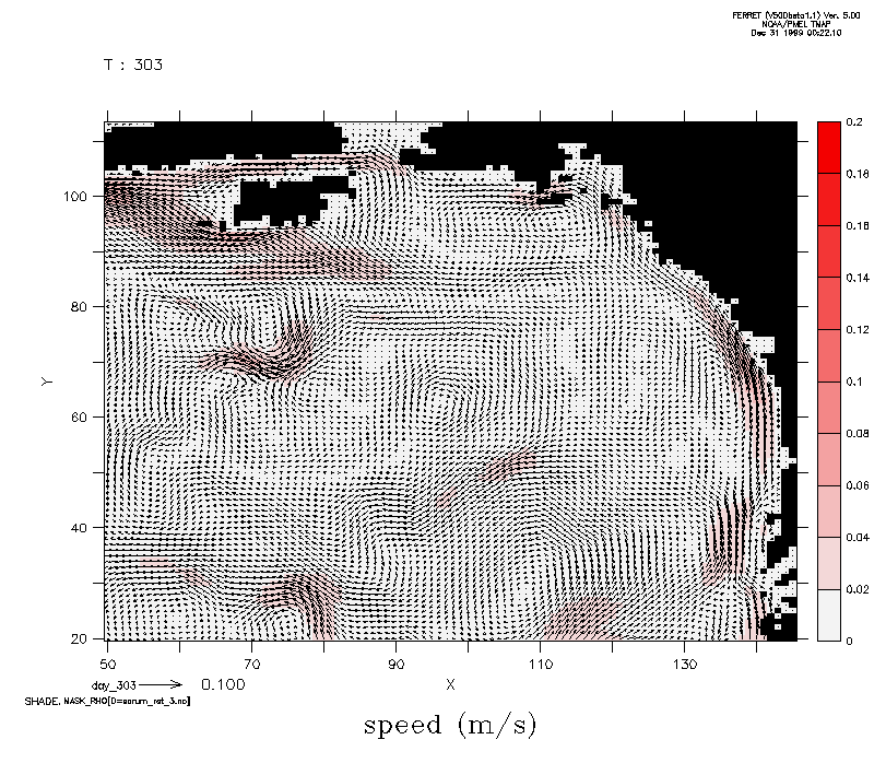
Fig. 15. Global model (SEOM) barotropic velocities (m/s) and speeds
(shaded, m/s) for DOY 303 1996.
A closeup of the Sitka region reveals far less structure than in the regional model; there is no clear "Sitka eddy".
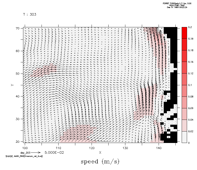
Fig. 16. Closeup of global model velocities and speeds in the vicinity
of Sitka AK.
By contrast, the regional model for the corresponding day exhibits a highly developed near-coastal eddy field associated with the Alaska Coastal Current. As noted in Fig. xx, buoyancy forcing is typically strongest in the fall, hence eddy generation via baroclinic insatability is a likely source of these smaller eddies. Larger meanders near the shelf break are also in evidence, but the smaller scale variability dominates. The Alaskan Stream appears considerably weaker, and sonewhat further offshore in this assimilating case, than was found in the non-assimilating regional run for early Novemeber 1976. A comparison of depth-integrated fluxes (not shown), similarly demonstrates weaker flux in this assimilating case than in the 1976 run.
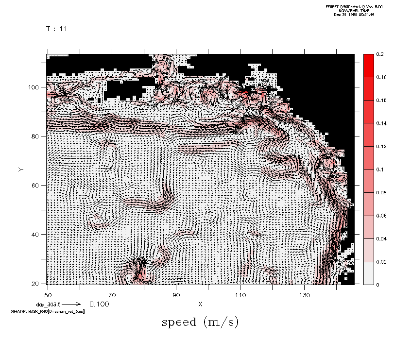
Fig 17. Regional model barotropic velocities (m/s) and speeds (m/s,
shaded) for DOY 303.5 1996. Global model barotropic velocities and climatological
T and S were used to spin up the regional model for DOY 210, and were subsequently
assimilated as a horinontal boundary condition for DOY 210-304.
A closeup of the Sitka region exhibits an eddy feature just southwest
of Sitka, similar to the one found in the non-assimilating 1976 run (see
Fig. xx). Near-coastal velocities are southeastward, in contrast to the
northwestward velocities of the global model (see Fig xx). This may be
a reflection of the more accurate, shallower bathymetry of the regional
model, with local daily winds exerting a stronger influence on the depth-integrated
currents. A time average of velocities for the previous 10 days (not shown)
in fact exhibits the more typical northwestward (that is, cyclonic around
the GOA) current pattern.
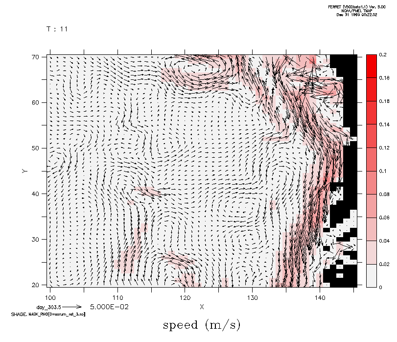
Fig. 18 Closeup of regional model velocities and speeds in the vicinity
of Sitka AK.
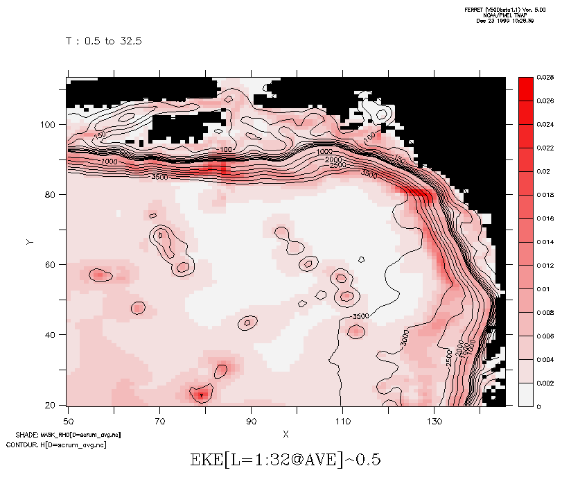
Fig. 19. RMS difference in regional model barotropic velocities, averaged over DOY 210-240, for two different assimilation schemes. In the first case, global model barotropic velocities and climatological T and S are assimilated at the horizontal boundaries. In the second case only climatological T and S were assimilated. Both runs were initially spun up with global model barotropic velocities for DOY 210.
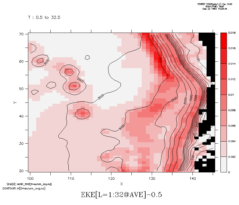
Fig. 20. Closeup of RMS difference between the two cases in the vicinity
of Sitka AK.
CONCLUSIONS!!!!!
(need to add)
References
Brodeur, R. D., B. W. Frost, S. R. Hare, R. C. Francis, and W. J. Ingraham, Jr. 1996. Interannual variations in zooplankton biomass in the Gulf of Alaska and covariation with California Current zooplankton. CalCOFI Reports, 37:80-99.
Chelton, D. B. and R. E. Davis. 1982. Monthly mean sea-level variability along the west coast of North America. J. Phys. Oceanogr. 12: 757-784.
Cummins, P. F. and L. A. Mysak 1988. A quasi-geostrophic circulation model of the Northeast Pacific. Part I: A preliminary numerical experiment. J. Phys. Oceanogr. 18:1179-1189.
Cummins, P. F. 1989. A quasi-geostrophic circulation model of the Northeast Pacific. Part II: Effects of topography and seasonal forcing. J. Phys. Oceanogr. 19:1649-1668.
Crawford, W. R., J. Y. Cherniawsky, and M. G. G. Foreman. 1999. Multi-year meanders and eddies in the Alaskan Stream as observed by the TOPEX/Poseidon altimeter. Submitted to Geophys. Res. Lett.
Haidvogel. 1999 ***need ref****
Haidvogel, D.B., E. Curchitser, M. Iskandarani, R. Hughes and M. Taylor. 1996. Global modeling of the ocean and atmosphere using the spectral element method. Atmosphere-Ocean, ***need update****
Hermann, A. J. and P. J. Stabeno. 1996. An eddy resolving model of circulation on the western Gulf of Alaska shelf. I. Model development and sensitivity analyses. J. Geophys. Res. 101: 1129-1149.
Hermann, A. J. and D. B. Haidvogel. 1999. Simultaneous Modeling of Tidal and Subtidal Dynamics in the Bering Sea. Extended abstract in *******
Lagerloef, G.S.E. 1995. Interdecadal variations in the Alaskan Gyre. J. Phys. Oceanogr. 25:2242-2258.
Melsom, A., S.D. Meyers, H.E. Hurlburt, E.J. Metzger and J.J. O'Brien. 1999. ENSO Effects on Gulf of Alaska Eddies, Earth Interactions, 3. [Available online at http://EarthInteractions.org]
Musgrave, D. L., T. J. Weingartner, and T. C. Royer. 1992. Circulation and hydrography in the northwestern Gulf of Alaska. Deep-Sea Res. 39: 14991519.
Milliff, R. F., W. G. Large, J. Morel, G. Danabasoglu and T. M. Chin. 1999. Ocean general circulation model sensitivity to forcing from scatterometer winds. J. Geophys. Res. 104: 11337-11358.
Reed, R. K. 1984. Flow of the Alaskan Stream and its variations. Deep Sea Res. 31:369386.
Reed, R. K., and J. D. Schumacher. 1989. Transport and physical properties in central Shelikof Strait, Alaska. Continental Shelf Res. 9:261268.
Reed, R.K., and S.J. Bograd. 1995. Transport in Shelikof Strait, Alaska: an update. Cont. Shelf Res.15:213218.
Royer, T.C. 1982. Coastal freshwater discharge in the northeast Pacific. J. Geophys. Res. 87:2017-2021.
Royer, T.C. 1983. Observations of the Alaska Coastal Current. pp. 9-30 in H.G. Gade, A. Edwards and H. Svendsen (eds.), Coastal Oceanography, Plenum Press.
Song, Y. and D. B. Haidvogel. 1994. A semi-implicit ocean circulation model using a generalized topography-following coordinate system. J. Comput. Res. 115:228-244.
Stabeno, P. J., R. K. Reed and J. D. Schumacher. 1995. The Alaskan Coastal Current, continuity of transport and forcing. J. Geophys. Res. 100:2477-2485.
Strub, P. T. and C. James. 1999. Altimeter-derived surface circulation in the large-scale NE Pacific gyres: Part 1. Annual variability. This volume.
Strub, P. T. and C. James. 1999. Altimeter-derived surface circulation in the large-scale NE Pacific gyres: Part 2. 1997-1998 El Nino anomalies. This volume.
Taylor, M., J. Tribbia, and M. Iskandarani. 1996. The spectral element method for the shallow water equations on the sphere. J. Comp. Phys., ***need update****
Tabata, S. 1982. The anticyclonic, baroclinic eddy off Sitka, Alaska, in the Norteast Pacific Ocean. J. Phys. Oceanogr. 12:1260-1282.
Thompson, R. E. and J. F. R. Gower. 1998 A basin-scale oceanic instability
event in the Gulf of Alaska. J. Geophys. Res. 103:3033-3040.